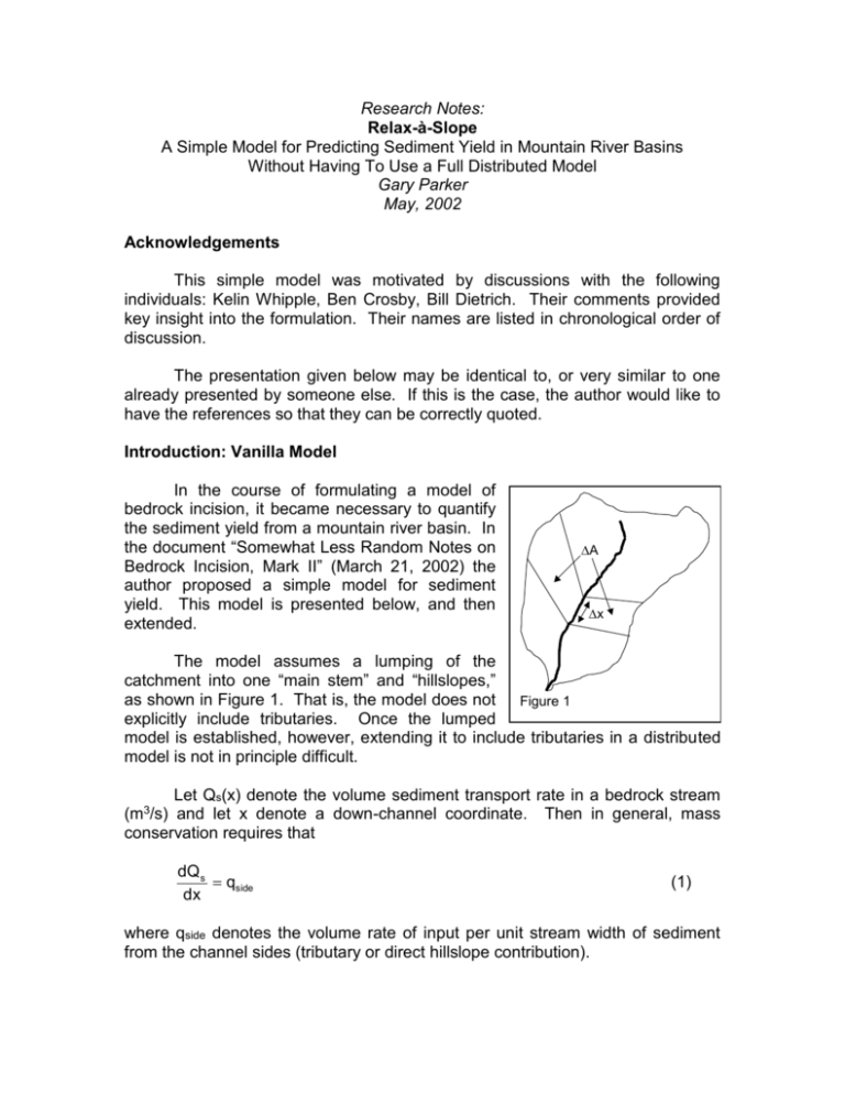
Research Notes:
Relax-à-Slope
A Simple Model for Predicting Sediment Yield in Mountain River Basins
Without Having To Use a Full Distributed Model
Gary Parker
May, 2002
Acknowledgements
This simple model was motivated by discussions with the following
individuals: Kelin Whipple, Ben Crosby, Bill Dietrich. Their comments provided
key insight into the formulation. Their names are listed in chronological order of
discussion.
The presentation given below may be identical to, or very similar to one
already presented by someone else. If this is the case, the author would like to
have the references so that they can be correctly quoted.
Introduction: Vanilla Model
In the course of formulating a model of
bedrock incision, it became necessary to quantify
the sediment yield from a mountain river basin. In
the document “Somewhat Less Random Notes on
Bedrock Incision, Mark II” (March 21, 2002) the
author proposed a simple model for sediment
yield. This model is presented below, and then
extended.
A
x
The model assumes a lumping of the
catchment into one “main stem” and “hillslopes,”
as shown in Figure 1. That is, the model does not Figure 1
explicitly include tributaries. Once the lumped
model is established, however, extending it to include tributaries in a distributed
model is not in principle difficult.
Let Qs(x) denote the volume sediment transport rate in a bedrock stream
and let x denote a down-channel coordinate. Then in general, mass
conservation requires that
(m3/s)
dQ s
 qside
dx
(1)
where qside denotes the volume rate of input per unit stream width of sediment
from the channel sides (tributary or direct hillslope contribution).
In the above-quoted document it was assumed that qside is simply
determined by the incision rate EI of the stream itself. Let A(x) denotes the
drainage area upstream of point x. If any streambed incision is assumed to
propagate instantaneously up the hillslope, it follows that
qsidex  EIA
(2a)
or thus, as illustrated in Figure 1,
qside  EI
dA
 EIBh
dx
(2b)
where
Bh 
dA
dx
(2c)
defines an effective basin “width” (from divide to divide) at point x.
Between the above relations it is found that
dQs
dA
 EI
dx
dx
(3)
The above equation gives a simple form for sediment yield in a drainage basin.
In the case of a steady-state landscape undergoing uplift at the constant rate , it
follows that EI is equal to , in which case (3) yields the result
Qs  A
(4)
Equation (3) is also able to capture sediment yield in a steady-state landscape
for which  is a function of x. In addition, it captures at least some features of
non-steady-state evolution. In particular, in the case for which EI is not equal to
, (3) allows the possibility for a sediment supply that changes as the nonsteady-state profile migrates upstream. Implicit in the model is the assumption
that whereas perturbations take a finite amount of time to propagate up the
channel, they propagate infinitely fast up the hillslopes (and by implication the
tributaries). This is not accurate in general, but may be good enough for some
purposes.
Problems with Vanilla Model
There are two main problems with the Vanilla Model of (3). The first is
that it does not distinguish between hillslopes and tributary catchments. As
pointed out above, this problem is easily remedied by extending the lumped
model of Figure 1, with one “main stem” and the rest treated as hillslopes, to a
distributed model that includes the tributaries.
The second problem is not so easily remedied. According to (2b), when
the incision rate falls to zero the sediment contribution from the sides drops to
zero as well. This cannot be true in general, because even after the cessation of
incision, hillslopes can contribute sediment to the channel by gradual lowering of
hillslope relief due to hillslope diffusion, or, as it were, diffusive hillslope
relaxation.
With this in mind, Vanilla Model is generalized to Relax-à-Slope as a way
to overcome this restriction.
Relax-à-Slope Formulation
Hillslopes are assumed to contribute sediment by two mechanisms;
hillslope diffusion and landsliding. Hillslope diffusion is described in terms of a
hillslope diffusivity  (m2/s). Landsliding is
described in terms of a limiting slope of the
hillslopes
hillslope Sl.
Various parameters are defined in
Figure 2. In particular,  denotes elevation
(e.g. on a hillslope). c denotes the
elevation of the channel, e denotes the
distance from the channel to the divide, and
y denotes a coordinate following the
hillslope drainage pattern from the divide to
the channel, such that y = (1/2) Bh denotes
the position of the channel.
e
channel
y

(1/2)Bh
c
Figure 2
The Exner equation of sediment
conservation in the channel is
 

(1   pb ) c     EI
 t

where t denotes time and pb denotes bedrock porosity (if any).
equation of sediment conservation on the hillslope is
q
 

(1   ph )
    h
y
 t

(5)
The Exner
(6)
where ph denotes the porosity of the hillslope regolith and qh denotes the volume
rate of transport of hillslope material down the hillslope per unit width (direction
normal to the hillslope drainage pattern).
Here the hillslope is assumed to have an “approximately” self-similar form;
  c
 fh ŷ  ,
e
ŷ 
y
1
Bh
2
(8)
where fh is a “universal” function. An example is a simple linear function;
fh  1 ŷ
(9)
Now (6) is integrated over the left hillslope in Figure 2;
(1  ph )
(1/ 2 )Bh
0
(1/ 2 )Bh
(1/ 2 )Bh q

h
dy  (1  ph )
dy  
dy
0
0
t
y
(10)
In order to complete the integration, it is assumed that  is constant in y, qh = 0 at
the ridge divide (y = 0) and Bh is constant in time (but not in x). Substituting (8)
into (10) and performing the integration, it is found that
1  
  1
(1  ph ) Bh  c  h1 e   (1   ph )Bn  qhc
2  t
t  2
(11)
where qhc = qh at y = (1/2)Bh = the sediment supply rate to the channel per unit
stream length, and h1 denotes an order-one dimensionless constant given by
the relation
1
h1   fh ( ŷ)dŷ
0
(12)
For example, in the case of the linear profile of (9) h1 =0.5.
Equation (11) can be further reduced with the aid of (5) and the
convenient assumption that pb = ph (which can be easily relaxed should one
desire), resulting in the form
1 
1
(1  ph )h1 Bh e  BhEI  qhc
2
t
2
An appropriate quantification for the slope of the hillslope S h is
(13)
Sh 
e
1
Bh
2
(14)
in which case (13) can be recast as
2
 1  dSh 1
(1   ph )h1 Bh 
 BhEI  qhc
2
 2  dt
(15)
Hillslope Sediment Delivery Rate
Assuming that the mechanism for the delivery of hillslope sediment is
hillslope diffusion, it follows that
qhc   

y y (1/ 2 )Bh
(16)
Here another implicit “similarity” assumption is introduced such that


 h2Sh
y y (1/ 2 )Bh
(17a)
where h2 is another order-one dimensionless parameter, obtained from (8) as
h2  
dfh
dŷ
(17b)
ŷ 1
.For example, for the linear profile of (9) h2 = 1. With (17a), (15) becomes
1 
1
(1  ph )h1 Bh e  BhEI  h2 Sh
2
t
2
(18)
Relax-à-Slope for Case of Hillslope Diffusion
Substituting (14) into (18) allows the definition of a relation governing
hillslope evolution:
2
 1  Sh 1
(1   ph )h1 Bh 
 BhEI  h2 Sh
2
 2  t
Equation (15) can then be recast as
(19)
2
1
 1  Sh
qhc  BhEI  (1   ph )h1 Bh 
2
 2  t
(20)
In the above formulation, the evolution of the hillslope is described using (19),
and the sediment delivery to the channel is computed from (20).
Remembering that qhc is the sediment delivery from the left side of the
channel according to Figure 2, so that in (1)
qside  2qhc
(21)
it follows from (19), (20) and (2c) that the extension of (3) is
2
dQs
dA
1  dA  Sh
 EI
 (1   ph )h1 

dx
dx
2  dx  t
(22)
where
2
1  dA  dSh
dA
(1   ph )h1 
 EI
 2h2 Sh

2  dx  t
dx
(23)
Equations (22) and (23) allow for a steady-state solution for which
dSh
0
dt
dQs
dA
qside 
 EI
dx
dx
1 EI dA
Sh 
2 h2  dx
(24a,b,c)
Note that (24b) reduces to exactly the same form as (4) under the assumption
that EI =  = a constant.
The real strength of the new method appears when EI is allowed to vanish.
In this case (22) and (23) reduce to
dQ s
 2h2 Sh
dx
(25)
2
1  dA  Sh
(1   ph )h1 
 2h2 Sh

2  dx  t
(26)
That is, even in the absence of incision, sediment supply from the hillslopes does
not fall to zero until Sh itself becomes vanishing. As the hillslopes relax under the
effect of hillslope diffusion in the absence of incision, a supply of sediment that
declines exponentially in time reaches the stream.
Extension to Landsliding
A very approximate extension of the formulation to encompass landsliding
can be accomplished in the following way. Let S l denote the limiting (maximum)
slope of the hillslope imposed by landsliding. One can assume that this limit is
reached at sufficiently high rates of channel incision, i.e. so high that they drive
repeated hillslope failure rather than diffusion. The simplest generalization of
(19) that realizes this is the form
 B
EI 
 1  Sh 1

(1  ph )h1 Bh 
 BhEI  h2 Sh 1  h
2
2


S
 2  t
h2
l 

(27)
2
In the limit of modest incision rates, or
Bh EI
 1
2 h2 Sl
(28)
(27) reduces to (19). On the other hand, in the limit of high incision rates, for
which
Bh EI

2 h2 Sl
(29)
(27) reduces to
 S 
 1  Sh 1
(1  ph )h1 Bh 
 BhEI 1  h 
2
Sl 
 2  t

2
(30)
which has the steady-state solution
Sh  Sl
In general, the steady-state solution is
(31)
Bh EI
2 h2 
Sh 
Bh EI
1
2 h2 Sl
(32)
The Full Model
The full model may thus be stated as
2
dQs
dA
1  dA  Sh
 EI
 (1   ph )h1 

dx
dx
2  dx  t
(33)

1  dA  Sh
dA
1 dA EI 

(1  ph )h1 
 EI
 2h2 Sh 1 

2  dx  t
dx
 2 dx h2 Sl 
(34)
2
The order-one coefficients h1 and h2 are dimensionless, order-one parameters
that can be specified for any given catchment based on field data, in accordance
with the definitions (8) (12), (14) and (17).