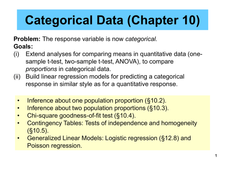
Categorical Data (Chapter 10)
Problem: The response variable is now categorical.
Goals:
(i) Extend analyses for comparing means in quantitative data (onesample t-test, two-sample t-test, ANOVA), to compare
proportions in categorical data.
(ii) Build linear regression models for predicting a categorical
response in similar style as for a quantitative response.
•
•
•
•
•
Inference about one population proportion (§10.2).
Inference about two population proportions (§10.3).
Chi-square goodness-of-fit test (§10.4).
Contingency Tables: Tests of independence and homogeneity
(§10.5).
Generalized Linear Models: Logistic regression (§12.8) and
Poisson regression.
1
Chi-Square Goodness-of-Fit Test
(§10.4)
Want to compare several (k) observed proportions (i), to
hypothesized proportions (io). Do the observed agree with the
hypothesized?
i = io, for categories i=1,2,...,k?
H0: i = io, for i=1,2,...,k
Ha: At least two of the observed cell proportions differ from the
hypothesized proportions.
2
Example: Do Birds Forage Randomly?
Mannan & Meslow (1984) studied bird foraging behavior in a forest in
Oregon. In a managed forest, 54% of the canopy volume was Douglas
fir, 40% was ponderosa pine, 5% was grand fir, and 1% was western
larch.
They made 156 observations of foraging by red-breasted nuthatches:
70 observations (45%) in Douglas fir; 79 (51%) in ponderosa pine; 3
(2%) in grand fir; and 4 (3%) in western larch.
Ho: The birds forage randomly.
Ha: The birds do NOT forage randomly. (Prefer certain trees.)
3
Bird Example: Summary
If the birds forage randomly, we would expect to find them in the
following proportions:
Douglas Fir
54%
Ponderosa Pine
40%
Grand Fir
5%
Western Larch
1%.
But the following proportions were observed:
Douglas Fir
45% (70)
Ponderosa Pine
51% (79)
Grand Fir
2% (3)
Western Larch
3% (4)
Do the birds prefer certain trees?
Perform a test using a Pr(Type I error)=0.05.
4
QUESTIONS TO ASK
What are the key characteristics of the sample data collected?
The data represent counts in different categories.
What is the basic experiment?
The type of tree where each of the 156 birds was observed
foraging was noted. Before observing, each has a certain
probability of being in one of the four types. After observing
they are placed in the appropriate class.
We call any experiment of n trials where each trial can have
one of k possible outcomes a Multinomial Experiment.
For individual j, the response, yj, indicates which outcome
was observed. Possible outcomes are the integers 1,2,…,k.
5
The Multinomial Experiment
•
•
•
•
•
The experiment consists of n identical trials.
Each trial results in one of k possible outcomes.
The probability that a single trial will result in outcome i is i
i=1,2,...,k, (Si=1) and remains constant from trial to trial .
The trials are independent (the response of one trial does not
depend on the response of any other).
The response of interest is ni the number of trials resulting in a
particular outcome i. (Sni=n).
Multinomial distribution: provides the probability distribution for the
number of observations resulting in each of k outcomes.
0!=1
n!
P(n1 , n2 ,, nk ) 
 1n1 2n2  knk
n1!n2! nk !
This tells us the probability of observing exactly n1,n2,...,nk.
6
From the bird foraging example
Hypothesized
Douglas Fir
Pond Pine
Grand Fir
West Larch
54%
40%
5%
1%
1=0.54
2=0.40
3=0.05
4=0.01
Observed
Douglas Fir
Pond Pine
Grand Fir
West Larch
n1=70
n2=79
n3=3
n4=4.
n!
P(n1, n2 ,, nk ) 
1n1 n22  nkk
n1!n2 !nk !
P(70,79,3,4) 
156!
(0.54)70 (0.4)79 (0.05)3 (0.01) 4
70! 79! 3! 4!
If this probability is high, then we would say that there is good
likelihood that the observed data come from a multinomial experiment
with the hypothesized probabilities. Otherwise we have the
probabilities wrong. How do we measure the goodness of fit between
the hypothesized probabilities and the observed data?
7
In a multinomial experiment of n
trials with hypothesized
probabilities of i i=1,2,...,k, the
expected number of responses in
each outcome class is given by:
A reasonable measure of
goodness of fit would be to
compare the observed class
frequencies to the expected
class frequencies. Turns out
(Pearson, 1900) that this statistic
is one of the best for this
purpose.
observed cell count
cell probability
Ei  n i , i  1,2,, k
expected cell count
2




n

E
2
i
i
  

Ei
i1 

k
Has Chi Square distribution with df = k-1 provided no sparse counts:
(i) no Ei is less than 1, and
(ii) no more than 20% of the Ei are less than 5.
8
Class
Douglas Fir
Pond Pine
Grand Fir
West Larch
2
Hypothesized
54% 1=0.54
40% 2=0.40
5% 3=0.05
1% 4=0.01
Observed
70
79
3
4
Expected
84.24
62.40
7.80
1.56
 ni  Ei 2 
Pr(Type I error  a = 0.05
 

E
i 1 
i

2
(70  84.24) (79  62.40) 2 (3  7.80) 2 (4  1.56) 2




84.24
62.40
7.80
1.56
k
 13 .5934
32,0.05  7.812
Since 13.59 > 7.81 we reject Ho.
Conclude: it is unlikely that the birds are foraging randomly.
(But: more than 20% of the Ei are less than 5… Use an exact test.)
9
R
> birds = chisq.test(x=c(70,79,3,4), p=c(.54,.40,.05,.01))
Chi-squared test for given probabilities
data: c(70, 79, 3, 4)
X-squared = 13.5934, df = 3, p-value = 0.003514
Warning message:
In chisq.test(x = c(70, 79, 3, 4), p = c(0.54, 0.4, 0.05, 0.01)) :
Chi-squared approximation may be incorrect
> birds$resid
[1] -1.551497
2.101434 -1.718676
1.953563
Looks like birds prefer Pond Pine & West Larch to the other two!
10
Summary: Chi Square Goodness of Fit Test
H0: i = i o for categories i=1,2,...,k
(Specified cell proportions for k categories)
Ha: At least two of the true population cell proportions differ from
the specified proportions.
Test Statistic:
2




n

E
2
i
i
  

E
i1 
i

k
Ei  i0  n
Rejection Region: Reject H0 if 2 exceeds the tabulated critical value
for the Chi Square distribution with df=k-1 and
Pr(Type I Error) = a.
11
Example: Genotype Frequency in Oysters
(A Nonstandard Chi-Square GOF Problem)
McDonald et al. (1996) examined variation at the CVJ5 locus in the
American oyster (Crassostrea virginica). There were two alleles, L and
S, and the genotype frequencies observed from a sample of 60 were:
LL: 14
LS: 21
SS: 25
Using an estimate of the L allele proportion of p=0.408, the HardyWeinberg formula gives the following expected genotype proportions:
LL: p2 = 0.167 LS: 2p(1-p) = 0.483
SS: (1-p)2 = 0.350
Here there are 3 classes (LL, LS, SS), but all the classes are functions
of only one parameter (p).
Hence, the chi-square distribution has only one (1) degree of freedom,
and NOT 3-1=2.
12
> chisq.test(x=c(14,21,25), p=c(.167,.483,.350))
Chi-squared test for given probabilities
R
data: c(14, 21, 25)
X-squared = 4.5402, df = 2, p-value = 0.1033
This p-value is WRONG! Must compare with chi-square with 1 df.
12,0.05  3.841
Since 4.5402 > 3.841, we should reject Ho.
Conclude that the genotype frequencies do NOT follow the HardyWeinberg formula.
13
Power Analysis in Chi-Square GOF Tests
Suppose you want to do a genetic cross of snapdragons with an
expected 1:2:1 ratio, and you want to be able to detect a pattern with
5% more heterozygotes than expected under Hardy-Weinberg.
Class
aa
aA
AA
Hypothesized
25% 1=0.25
50% 2=0.50
25% 3=0.25
Want to detect (from data)
22.5%
55%
22.5%
The necessary sample size (n) to be able to detect this difference can be
computed by the more comprehensive packages (SAS, SPSS, R). There is
also a free package, G*Power 3 (correct as of Spring 2010):
[http://www.psycho.uni-duesseldorf.de/abteilungen/aap/gpower3/
Inputs: (0.25,0.50,0.25) for hypothesized; (0.225,0.55,0.225) for expected;
and df=1. Should get n of approx 1,000.
14
Tests and Confidence Intervals
for One and Two Proportions
(§10.2, 10.3)
First look at case of single population proportion ().
A random sample of size n is taken, and the number
of “successes” (y) is noted.
15
Binomial Experiment = Multinomial Experiment with two classes
n!
P(n1, n2 ) 
1n1 n22
n1!n2 !
1  
Since the sum of the proportions is equal to
1, we have:
2  (1  )
Since the sum of the cell frequencies equal the total n  y
1
sample size.
n2  (n  y)
P( y | n, ) 
n!
 y (1  )n y
y! (n  y)!
If  is the probability of a “success” and y
is the number of “successes” in n trials.
Estimate of success probability is:
y
ˆ 
n
16
Normal Approximation to the Binomial and CI for 
In general, for n    5 and n  (1 )  5
the probability of observing y or greater successes can be
approximated by an appropriate normal distribution (see section 4.13).
Pr(Y  y)  Pr(Z  z ),
Z ~ N (0,1),
z
y  n
n (1   )
What about a confidence interval (CI) for ?
Using a similar argument as for y, we obtain the (1-a)100% CI:
ˆ  z a  ˆ
2
y
ˆ 
n
 ˆ 
(1  )
n
Use
ˆ ˆ 
ˆ (1  ˆ )
n
when  is unknown.
17
Approximate Statistical Test for 
H0:  = 0 (0 specified)
Test Statistic:
Ha:
ˆ  0
z
ˆ
1.
2.
3.
Note: Under H0:
 ˆ 
Rejection Region:
1.
2.
3.
 > 0
 < 0
  0
0 (1  0 )
n
Reject if z > za
Reject if z < -za
Reject if | z | > za/2
18
Sample Size needed to meet a pre-specified confidence in 
Suppose we wish to estimate  to within  E with confidence
100(1-a)%. What sample size should we use?
z a 2 (1  )
2
n
E2
Since  is unknown, do the following:
1.
Substitute our best guess.
2.
Use  = 0.5 (worst case estimate).
Example:
We have been contracted to perform a survey to determine what
fraction of students eat lunch on campus. How many students should we
interview if we wish to be 95% confident of being within  2% of the true
proportion?
Worst case:
( = 0.5)
Best guess:
( = 0.2)
1.962 0.5  (1  0.5) 3.8416 0.25
n

 2401
2
0.02
.0004
1.962 0.2  (1  0.2) 3.8416 0.16
n

 1475
2
0.02
.0004
19
Comparing Two Binomial Proportions
Situation: Two sets of 60 ninth-graders were taught algebra I by
different methods (self-paced versus formal lectures). At the end
of the 4-month period, a comprehensive, standardized test was
given to both groups with results:
Experimental group:
n=60, 39 scored above 80%.
Traditional group:
n=60, 28 scored above 80%.
Is this sufficient evidence to conclude that the experimental group
performed better than the traditional group?
Each student is a Bernoulli trial with probability 1 of success (high
test score) if they are in the experimental group, and 2 of success if
they are in the traditional group.
H 0: 1 = 2
versus
H a: 1 >  2
20
Population proportion
Sample size
Number of successes
Population
1
2
1
2
n1
n2
y1
y2
Example
60
39
yi
0.65
ˆ i 
Sample proportion:
ni
100(1-a)% confidence interval for 1 - 2.
ˆ 1  ˆ 2  z a 2 ˆ 1 ˆ 2
ˆ 1 ˆ 2 
1(1  1) 2 (1  2 )

n1
n2
Ex: 90% CI is
60
28
0.467
use
ˆi for  i
0.183 ± 1.645(0.089)  (.036, .330)
21
Interpret …
Statistical Test for Comparing Two Binomial Proportions
H0: 1 - 2 =0 (or 1 = 2 = 
Ha:
ˆ 1  ˆ 2
z
ˆ 1 ˆ 2
Test Statistic:
1.
2.
3.
1 - 2 > 0
1 - 2 < 0
1  2  
Note: Under H0:
 ˆ ˆ 
1
2
Rejection Region:
ˆ1 (1  ˆ1 ) ˆ 2 (1  ˆ 2 )
n1

1.
2.
3.
n2
Reject if z > za
Reject if z < -za
Reject if | z | > za/2
22
Population proportion
Sample size
Number of successes
Population
1
2
1
2
n1
n2
y1
y2
Example
60
39
Sample proportion:
ˆ1  0.65,
Test Statistic:
0.65
ˆ2  0.467,
0.467
ˆˆ ˆ  0.089
1
2
ˆ1  ˆ 2 0.65  0.467
z

 2.056
 ˆ ˆ
0.089
1
z0.05  1645
.
60
28
2
Since 2.056 is greater than
1.645 we reject H0 and
conclude Ha: 1 > 2.
23