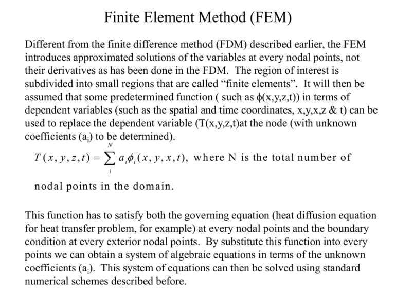
Finite Element Method (FEM)
Different from the finite difference method (FDM) described earlier, the FEM
introduces approximated solutions of the variables at every nodal points, not
their derivatives as has been done in the FDM. The region of interest is
subdivided into small regions that are called “finite elements”. It will then be
assumed that some predetermined function ( such as (x,y,z,t)) in terms of
dependent variables (such as the spatial and time coordinates, x,y,x,z & t) can be
used to replace the dependent variable (T(x,y,z,t)at the node (with unknown
coefficients (ai) to be determined).
N
T ( x, y, z, t) 
 a  ( x , y , x , t ),
i
i
w here N is the total num ber of
i
nodal points in the dom ain.
This function has to satisfy both the governing equation (heat diffusion equation
for heat transfer problem, for example) at every nodal points and the boundary
condition at every exterior nodal points. By substitute this function into every
points we can obtain a system of algebraic equations in terms of the unknown
coefficients (ai). This system of equations can then be solved using standard
numerical schemes described before.
Finite Element Example
Determine the temperature distribution of the flat plate as shown below using
finite element analysis. Assume one-dimensional heat transfer, steady state, no
heat generation and constant thermal conductivity. The two surfaces of the plate
are maintained at constant temperatures of 100°C and 0°C, respectively.
T=100°C
T=0°C
x2=3/2
x1=1/2
x3=5/2
1
2
First, divide the plate into three elements (1,2
& 3). The temperatures of these three
elements are represented by their nodal
temperatures T1,T2 & T3, respectively.
Next, assume the temperature is a function of
its coordinate: T(x)=Ax2+Bx+C. A,B & C are
three constants.
3
Finally, determine the constants using the
governing equation and all corresponding
boundary conditions.
L=3
Example (cont.)
To simplify the solution, we can apply the governing equation first:
 T
2
 T  0,
2


2
( Ax  Bx  C )  2 A  0
2
x
x
Therefore, A=0 for all nodal temperature functions. This is no surprise for us
since we know the steady state, no generation, 1-D heat transfer should have a
linear temperature distribution. Therefore: T(x)=Bx+C and the three nodal
equations are:
T1=Bx1+C=(B/2)+C, T2=Bx2+C=(3B/2)+C, T3= Bx3+C=(5B/3)+C
2
2
Therefore, there are only two constants to be solved and they can be determined
using the two boundary conditions. At the left-side surface, the temperature is a
constant 100°C and there is a constant heat transfer into the element 1 and the
same amount of the heat is transferred to the element 2 since there can be no heat
accumulation inside the element to satisfy the steady state condition.
q(left surface to element 1) = q(element 1 to element 2)
Example (cont.)
k
100  T1
x1  0
k
T1  T 2
x 2  x1
,
100  T1

T1  T
1/ 2
1
B
  3B

3T1  T 2  200, 3   C   
 C   200
 2
  2

0( B )  2 ( C )  200: T he first equation
zero
The second equation can be determined by using the boundary condition
on the other side of the plate:
k
T2  T3
x3  x2
k
T3  0
3  x3
,
T2  T3
1

T3
1/ 2
 5B
  3B

3T 3  T 2  0, 3 
C
C0
 2
  2

6 B  2 C  0 : T he second equation
Example (cont.)
T he finite elem ent m atrix for the consta nts B & C is:
0

6
2   B   200 
   

2  C   0 
S olve using any num erical schem e: B = -
100
, C  1 00
3
T ( x )  100 
100
x
3
This equation satisfies both boundary conditions: T(x=0)=100°C and
T(x=3)=0 °C.
For most finite element problems, we have to use thousands or even
millions of elements in order to resolve as much detailed information as
possible. Therefore, a fast numerical solver for the matrix (system of
equations) is necessary to obtain satisfactory results. The use of numerical
scheme has been discussed previously when we introduce the finite
difference method.