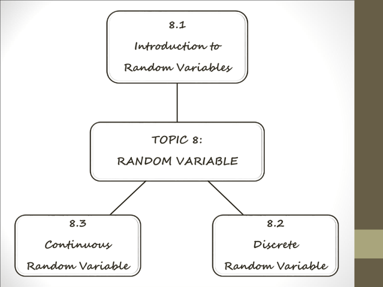
8.1
Introduction to
Random Variables
TOPIC 8:
RANDOM VARIABLE
8.3
8.2
Continuous
Discrete
Random Variable
Random Variable
8.1
Introduction to
Random
Variables
At the end of the lesson, students should be able to:
 Understand the concept of discrete and continuous
random variables.
is defined as a characteristics or
attribute that can assume different
values.
VARIABLE
various alphabet, such as X, Y
or Z used to represent
variables.
Example..
If two coins are tossed, a letter
‘y’ can be used to represent
the number of heads, in this
case, 0,1 or 2.
* Since the variables are associated with probability, they are
called random variables.
RANDOM
VARIABLES
• is a variable whose values (a real
number) depends on the outcome
of a random experiment
Example : Consider an experiment of tossing a coin twice,
The outcome of the experiment can be listed as a
sample space,
S = {HH, HT, TH, TT} where H = Head, T = Tail
Let X , the variable being considered is number of
heads obtained. The number of heads obtained in this
case could be 0, 1 or 2. The probability of these
occurring are as follows..
P  no heads   P TT 
  0.5  0.5 
 0.25
P  one head   P  HT   P TH 
  0.5  0.5    0.5  0.5 
 0.5
P  two heads   P  HH 
  0.5  0.5 
 0.25
We can show the results in a table, known as
probability distribution.
Number of
heads
Probability
0
1
2
0.25
0.5
0.25
The probabilities can be written as,
P  X  0  0.25, P  X  1  0.5, P  X  2  0.25
There are 2 types of random variables:-
Discrete Random
Variable
• If it has finite or
countable number of
possible outcomes that
can be listed
• Represent count data
Continuous
Random Variable
• If it has an uncountable
number of possible
outcomes represented by
an interval on the number
line
• Represent measured
data
EXAMPLES…
Discrete Random Variable
Continuous Random
Variable
Number of children
in a family
Weights of persons
in a company
Number of patients
in a doctor’s surgery
Heights of students
in a school
Number of students
in KMM
Time required to run
a mile
EXERCISE
Indicate which of the following random variables are
continuous or discrete:
(a) The life of a battery
(b) The number of new accounts opened at bank during a
certain month
(c) The time spend by students in answering a question
(d) The price of a concert ticket
(e) The number of rooms in a house
8.2
Discrete
Random
Variables
At the end of the lesson, students should be able to:
 Construct probability distribution table and
probability distribution function.
① PROBABILITY DISTRIBUTION FUNCTION
If X is a discrete random variable which takes values,
x1 , x2 , x3 ,..., xn
then
P  X  xi 
is the respective probability of X, that is
P  X  x1  , P  X  x2  , P  X  x3  ,..., P  X  xn 
REMEMBER!!!
The probability distribution of a discrete random variable
have the following characteristics:(a)
0  P X  1
n
(b)
for each value of
P X  x  1
i 1
i
x
EXAMPLE 1:
Construct the probability distribution function, if two
fair coins are tossed.
EXAMPLE 2:
For the following probability distribution function, find
the values of a .
P  X  x   ax, for x  1,2,3,4
EXAMPLE 3:
Given the discrete random variable X has the following
probability distribution function.
2 px , x  0,1, 2
g  x  
 px , x  3, 4
Where p is a constant. Find the value of p . Hence,
sketch the graph of g  x 
EXAMPLE 4:
A fair die is rolled. If X represents the number on die,
show that X is a discrete random variable. Find
P  X  5 and P 1  X  4 .
EXAMPLE 5:
The probability distribution function of a discrete
random variable X is given by
P  X  x   kx2
Where x  0,1, 2,3, 4
(a) Find the value of the constant, k
(b) Construct the probability distribution table
(c) Find
(i) P  X  1 or X  4
(ii) P X  2  1


EXAMPLE 6:
The random variable Y has a probability
12  y
P Y  y  
36
for y  0, 2, 4,6
(a) Construct the probability distribution table for Y
(b) Draw the graph for the probability distribution of Y
(c) Find P Y  2
EXAMPLE 7:
The discrete random variable W has a probability
a

P W  w   a  b
b

for w  0,1
for w  2
for w  3, 4
5
If P W  2   , find the values of a and b
9
Let’s try this!!
The discrete random variable U has a probability
u
for u  2,3,5
 2k

u
P U  u   
for u  7,8,10
 5k
otherwise
0


Find the value of k . Hence,
ANS:
k  10
(a) Construct a probability distribution table for U
(b) Find P  4  U  8
ANS: 0.55
8.2
Discrete
Random
Variables
At the end of the lesson, students should be able to:
 find the cumulative distribution function and solve
related problems.
② CUMULATIVE DISTRIBUTION FUNCTION
Let us revise back….
In Chapter 6..if given a frequency distribution,
corresponding cumulative frequencies are
obtained by summing all the frequencies up to a
particular value..
 similarly, if X is a discrete random variable, the
corresponding cumulative probabilities are
obtained by summing all probabilities up to a
particular value.
If X is a discrete random variable with distribution function
P  X  xi  for x  x1 , x2 , x3 ,..., xn ,
then the cumulative distribution is given by
F  x  P  X  x
x
  P  X  x
x1
F  x
where:-
EXAMPLE 1:
Complete the cumulative distribution table below for
random variable X where X is the score on an unbiased
dice.
SOLUTION:
x
1
2
3
4
5
6
P  X  x
1
6
1
6
1
6
1
6
1
6
1
6
EXAMPLE 2:
The probability distribution for random variable X is
shown in the table. Construct the cumulative
distribution table and sketch the graph for cumulative
distribution function.
1
2
3
0
x
P  X  x  0.03 0.04 0.06 0.12
4
0.4
5
0.15
6
0.2
EXAMPLE 3:
The cumulative distribution function F  x  of a discrete
random variable X is defined as follows:
0
1

5
 8
F  x  
15
4
5

1
,
x2
, 2 x3
,
3 x  4
,
4 x5
,
x5
(a) Find
(i)
P  X  3
(ii)
(iii)
P  X  3
P  X  3
(iv) P  X  3
(v)
(vii) P  3  X  5
(ix)
P  2  X  4
(vi)
P  X  3
P 3  X  5
(viii) P  2  X  4
(b) Find the probability distribution function.
EXAMPLE 4:
The cumulative distribution function F  x  of a discrete
random variable X is shown as below:
x
F  x
Find
(a) P  X  3
(b) P  X  2
(c) P  2  X  4
1
2
3
4
0.2
0.32
0.67
0.9
5
1
EXAMPLE 5:
The cumulative distribution function F  x  of a discrete
random variable X is shown as below:
0
a

3a
F  x  
8a
12a

1
,
x 1
,
1 x  3
,
3 x5
,
5 x7
,
7 x9
,
x9
3
Given P  4  X  8   . Find the value of a . Hence,
5
find the probability distribution function.
Let’s try this!!
The discrete random variable X has the following
probability distribution function:
1
6

1
f  x  
3
0


, x  0, 2
, x  1,3
, otherwise
Find the cumulative distribution function, F  x  and
sketch its graph. Hence, find
Hence, find
(a) P  X  2
(b)
P  X  1
(c)
P  0  X  3
(d)
P  X  2
(e)
P  X  1
2
,
ANS:  a 
3
1
5
 b  , (c) ,
6
6
1
1
 d  , (e)
3
2
8.2
Discrete
Random
Variables
At the end of the lesson, students should be able to:
 find mean and variance
③ EXPECTATION AND VARIANCE
(A) EXPECTATION
Expectation or the expected value of a random variable
X is mean of X and is denoted by,
(I)
EX   
If X is a discrete random variable with probability
distribution function, P  X  x  , then
(2)
 x  P  X  x
If g  X  is a function of a discrete random variable
X, then the expectation of g  X  is defined as
follows:
(3)
E  g  X     g  X   P  X  x 
For expectation of X 2 ,
(4)
x
2
 P  X  x
If a and b are constants,
 E a  a
(5)
 E  aX   aE  X 
 E  aX  b   a  E  X   b
EXAMPLE 1:
The probability distribution of a discrete random
variable X is given as follows.
x
1
2
3
4
5
P  X  x
0.1
0.3
0.3
0.2
0.1
Calculate E  X 
EXAMPLE 2:
The discrete random variable X has the following
probability distribution :
x
1
2
t
P  X  x
0.1
0.2
0.7
Find the value t if E  X   4
EXAMPLE 3:
The probability distribution of a discrete random
variable X is given in the table below:
Find:(a) E  2 
x
1
2
3
P  X  x
1
6
2
6
3
6
(d)
E  5 X  2
(b)
EX 
(e)
EX2
(c)
E 5X 
(f)
E 5 X 2  2
EXAMPLE 4:
X is a discrete random variable and k is a constant. If
E 3X  k   26 and E  2k  X   3 , find the value of
k and E  X  .
EXAMPLE 5:
X is a discrete random variable and given E  X   5.
Find
(a) E 5 X  4
(b)
3
E Y  if Y  X  1
2
Let’s try this!!
A discrete random variable can only take values 2 and 3
and has expectation 2.6. Find the probabilities
P  X  2 and P  X  3
ANS : P  X  2  0.4 , P  X  3  0.6
(B) VARIANCE
   E  X 
① Var  X   E X
2
2
② If a and b are constants,
Var  a   0
Var  aX   a
2
Var  X 
Var  aX  b   a Var  X 
2
Var  aX     a  Var  X 
2
③ The standard deviation,
  Var  X 
TAKE NOTE!!
Variance always positive!
EXAMPLE 1:
The probability distribution of a discrete random
variable X is given as follows:
1
x
P  X  x
 
2
7
2
3
4
7
1
7
Calculate E  X  , E X 2 , Var  X 
EXAMPLE 2:
The probability distribution of a discrete random
variable X is given as follows:
x
1
2
3
4
P  X  x
1
16
1
2
1
4
3
16
Find
(a) Var  X 
(b) Var  X  2
(c) Var  2 X  2
(d) Var  5  8 X 
8.3
Continuous
Random
Variables
At the end of the lesson, students should be able to:
 Identify the probability density function
 Determine the probability from a probability
density function
① PROBABILITY DENSITY FUNCTION
A continuous random variable X takes
any value within a range or INTERVAL.
The probabilities can be found from the
probability density function, f x by


b
P  a  X  b    f  x  dx
a
If
f  x  0

for all x and
 f  x  dx  1

As P
then,
 X  k   0 , where k
is constant,
P  a  X  b  P  a  X  b
 P  a  X  b
 P  a  X  b
Unlike discrete distribution, we
do not need to worry EQUAL
SIGN!
EXAMPLE 1:
A continuous random variable X has probability density
function, f  x   kx3 for 0  x  4 . Find
(a) the value of the constant k
(b) P 1  X  3
EXAMPLE 2:
A continuous random variable X has probability density
1
function, f  x    4  x  for 1  x  3 .
4
(a) Verify that it satisfies the condition of a probability
density function.
(a) Find P  X  2
EXAMPLE 3:
Given the continuous random variable X has the
following probability density function:
kx 2
f  x 
, 4 x  4
2
3
Show that k 
. Hence, find
64
(a) P  X  2
(b) P  X  3
(c) P  2  X  1
(d) P  0  X  3
(e) P  1  X  1
(f) P  X  2
EXAMPLE 4:
X is a continuous random variable with probability
density function:
 x  1 , 0  x  1


f  x   x 1
, 1 x  2

, otherwise

0
Find
(a) P 1  X  2
(b) P  X  1.5
5
1
(c) P   X  
4
4
Let’s try this!!
The continuous random variable X has probability
density function
h , 2 x4

f ( x)  kx , 5  x  6
 0 , otherwise

1
Given P  X  3  . Find the values h and k.
8
1

Hence , find P  X  3 
2

ANS :h 
1
3
1  13

,k
, P X  3  
8
22
2  16

8.3
Continuous
Random
Variables
At the end of the lesson, students should be able to:
 Find the cumulative distribution function and solve
related problems.
② CUMULATIVE DISTRIBUTION FUNCTION
Cumulative
distribution function
for a continuous
random variable X
with probability
density function, f  x 
is
F(x) is the area under the curve
y  f  x  from  up to x as
indicated below
y
y  f  x
F  x  P  X  x
x

 f  x  dx

x
x
NOTES!!
★ P  X  a  P  X  a  F a
★ P  a  X  b  F b   F  a 
Remember!!
P  a  X  b  P  a  X  b
 P  a  X  b
 P  a  X  b
EXAMPLE 1:
X is a continuous random variable with probability
1
density function, f  x   x for 0  x  4 . Find the
8
cumulative distribution function.
EXAMPLE 2:
The probability density function of a continuous random
variable X is defined as,
2
3
16  x  2 

2
3
f  x     x  2
16
0


,
2 x 0
, 1 x  2
,
otherwise
(a) Obtain the cumulative distribution function
EXAMPLE 3:
The continuous random variable X has the cumulative
distribution function given by
,
0
 2x

,
5
F  x  
2

4
2
x
   3 x   4  ,
5 5 
2


,
1
(a) P  X  0.5
x0
0 x2
2 x3
(b) P 1  X  2.5
x3
Let’s try this!!
 ax , 0  x  1
1
f ( x)   a3  x  , 1  x  3
2
 0 , otherwise
Find
(a) the value of a


(c) P  X  1 
1

2
(b) F(x)
58
A continuous random variable X has the following
probability density function
ANSWERS:
2
(a) a 
3
0
1
 x2
3
(b) F ( x)  
2
x
1
x 


6 2

1
,
x0
,
0  x 1
,
1 x  3
,
x3
1

(c) P  X  1    0.5417
2

F  x    f  x  dx
Probability
Density
Function
Cumulative
Distribution
Function
d
f  x 
F  x
dx
EXAMPLE 1:
A continuous random variable has a cumulative
distribution function given by,
0
 3
x
F  x  
 27
1
,
x0
,
0 x3
,
x3
Obtain the probability density function.
EXAMPLE 2:
The cumulative distribution function of a continuous
random variable X is defined as follows:
0
1
 2  x
12

x
F  x   a 
6

x

b  12

1
,
x  2
,
2 x 0
,
0 x4
,
4 x6
,
x6
(a) Find a and b
(b) Determine the probability density function, f  x 
(c) Calculate P 3  X  5
8.3
Continuous
Random
Variables
At the end of the lesson, students should be able to:
 Find the mean and variance
③ EXPECTATION AND VARIANCE
(A) EXPECTATION
FYI..Expectation also known as the
mean / average for random variable
★ If X is a continuous random variable with probability density
function, f  x  , then
◤

  EX  

x f  x  dx


◥   
E X2 

x2 f  x  dx
★ If X is a continuous random variable with probability density
function, f  x  , then

◤ E  g  X    g  x 
f  x  dx

If a and b are constants,
E  a  a
E aX   a E  X 
E aX  b  a E  X   b
EXAMPLE 1:
Given the continuous random variable X has the
following probability density function:
3

4  x  x 
f  x  

0
Find E  X 
,
0  x 1
,
otherwise
EXAMPLE 2:
Given the continuous random variable X has the
following probability density function:
x
,
3

 1
,
f  x  3
1
 4  x ,
3
0
,
Find E  X 
0  x 1
1 x  3
3 x  4
otherwise
EXAMPLE 3:
Given the continuous random variable X has the
following probability density function:
x5

f  x    50

0
,
5  x  5
,
otherwise
Find
(a) E  X 
(c) E 3X  2
(b) E X 2
(d) E 2 X 2  5 X  1
 


(B) VARIANCE
   E  X 
  Var  X   E X
2
2
If a and b are constants,
Var  a   0
Var  aX   a Var  X 
2
Var  aX  b   a 2Var  X 
2
EXAMPLE 1:
Given the probability density function:
4
 3 1  x 

4
f  x   x
3
0


1
, 0 x
2
1
,
 x 1
2
, otherwise
Calculate Var  X . Hence, find the standard deviation
of X.
EXAMPLE 2:
X is a continuous random variable with probability
density function, f  x  . If


x 2 f  x  dx  29 and

Var  3X   36 , find the mean of X.
EXAMPLE 3:
Given probability density function
3
f  x   1  x 2  , 0  x  1
4
If E  X    and Var  X    2 , find P  X     