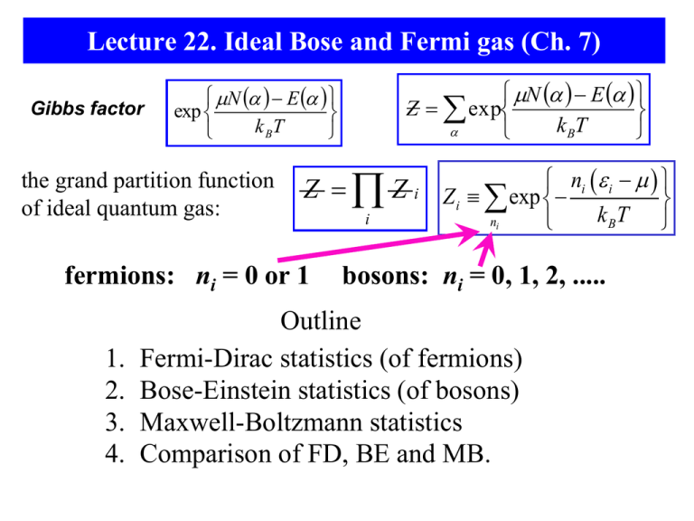
Lecture 22. Ideal Bose and Fermi gas (Ch. 7)
Gibbs factor
the grand partition function
of ideal quantum gas:
Z   Z i Zi   exp  ni  i    
fermions: ni = 0 or 1
1.
2.
3.
4.
 N    E   
Z   exp

k BT



 N    E   
exp 

k
T
B


i
ni

kBT
bosons: ni = 0, 1, 2, .....
Outline
Fermi-Dirac statistics (of fermions)
Bose-Einstein statistics (of bosons)
Maxwell-Boltzmann statistics
Comparison of FD, BE and MB.

The Partition Function of an Ideal Fermi Gas
The grand partition function for all particles in the ith
single-particle state (the sum is taken over all possible
values of ni) :
 ni    i 
Z i   exp

ni
 k BT 
   i
 1  exp 
 k BT



If the particles are fermions,
n can only be 0 or 1:
Z
Putting all the levels
together, the full partition
function is given by:

    i 

  1  exp
i 
 k BT  
Z FD
FD
i
Fermi-Dirac Distribution
The probability of a state to be occupied by a fermion:
 ni    i 
1
P i , ni   exp
ni  0, 1

Zi
 k BT 
The mean number of fermions in a particular state:
1 
1

ni 
Zi 
1  exp       i 
 Zi 
1  exp       i  


exp       i 
1  exp       i 


1
exp    i     1
Fermi-Dirac distribution
( is determined by T
and the particle density)
1
nFD   
  
  1
exp
 k BT 
Fermi-Dirac Distribution
At T = 0, all the states with  < 
have the occupancy = 1, all the
states with  >  have the
occupancy = 0 (i.e., they are
unoccupied). With increasing T, the
step-like function is “smeared” over
the energy range ~ kBT.
1
~ kBT
0
T=0
(with respect to )
=
The macrostate of such system is completely defined if we
know the mean occupancy for all energy levels, which is
often called the distribution function:
f E   n E 
While f(E) is often less than unity, it is not a probability:
 f E   n
i
n=N/V – the average
density of particles
The Partition Function of an Ideal Bose Gas
The grand partition function for all particles in the ith
single-particle state (the sum is taken over all possible
values of ni) :
 ni     i  
Zi   exp 

k
T
ni
B


If the particles are Bosons, n can be any #, i.e. 0, 1, 2, …
 ni     i  
    i  
 2    i  
Zi   exp 
  1  exp 
  exp 

ni  0
 k BT 
 k BT 
 k BT 


2
If
x

1,
1

x

x


1 

1  x 
Zi
BE

   i
 1  exp 
 k BT

Putting all the levels

   i
together, the full partition Z BE   1  exp 
i 
 k BT
function is given by:






1
1
  min i 
Bose-Einstein Distribution
The probability of a state to be occupied by a Boson:
 ni     i  
1
P  i , ni   exp 
 ni  0,1,2,
Zi
 k BT 
The mean number of Bosons in a particular state:
1

    i  
1

ni 
Zi  1  exp 
1  exp       i 


Zi    
 k BT      


   i
 1  exp 
 kBT

  exp       i 

  1  exp       i 

Bose-Einstein distribution

2

1
exp    i     1
  min  
The mean number of particles in a
1
nBE   
given state for the BEG can exceed
  
exp 
 1 unity, it diverges as   min().

 k BT 
Comparison of FD and BE Distributions
2
1
nFD   
  
  1
exp
 k BT 
<n>
BE
1
FD
nBE   
n n
0
-6
when
-4
 
k BT
-2
0
2
()/kBT
  
1, exp 

k
T
 B 
Maxwell-Boltzmann
distribution:
4
1
6
1
  
exp 
1

 k BT 
nFD    nBE   
nMB   
1
  
exp 

k
T
 B 
1
  
exp 

k
T
 B 
Maxwell-Boltzmann Distribution (ideal gas model)
Recall the Boltzmann distribution (ch.6) derived from canonical ensemble:
 2 mk B T 
Z1  V 

2
h


3/ 2
V

VQ
  V
1 N
Z
Z1 F  k BT ln Z   Nk BT ln 

N!
  NVQ
 V
 F 
 
  k BT ln 
 N T ,V
 NVQ
 1 N
N

ln

 exp   

 
Z1
   Z1 
 
  1
 
The mean number of particles in a particular state of N particles in
volume V:
nMB    N  P   
N
exp      exp    exp      exp       
Z1
  
nMB    exp  
MB is the low density limit where the

k
T
B


difference between FD and BE disappears.
Maxwell-Boltzmann distribution
nVQ
1 i.e. N Z1
1 and   0
nVQ  1
Comparison of FD, BE and MB Distribution
2
<n>
MB
1
nFD   
  
  1
exp
 k BT 
BE
1
1
nBE   
  
exp 
1

 k BT 
FD
n n
0
-6
-4
-2
0
2
()/kBT
4
6
  
nMB    exp  

k
T
B


what are the possible values of MB , FD , and BE ? assume   0
MB  0
FD   F   0
BE  min    0
Comparison of FD, BE and MB Distribution
(at low density limit)
<n>
1.0
 = - kBT
The difference between FD, BE
and MB gets smaller when  gets
more negative.
MB
FD
BE
0.5
i.e., when 
0.0
0
1
/kBT
2
3
MB is the low density limit where
the difference between FD and BE
disappears.
0.2
MB
FD
BE
<n>
 = - 2kBT
0.1
nVQ
0.0
0
1
2
/kBT
0, nFD  nBE  nMB
3
1 i.e. N Z1
1
Comparison between Distributions
Boltzmann
nk 
1
  

exp
 k BT 
Bose
Einstein
nk 
1
  
  1
exp
 k BT 
Fermi
Dirac
nk 
1
  
  1
exp
 k BT 
indistinguishable
Z=(Z1)N/N!
nK<<1
indistinguishable
integer spin 0,1,2 …
indistinguishable
half-integer spin 1/2,3/2,5/2 …
spin doesn’t matter
bosons
fermions
localized particles
 don’t overlap
wavefunctions overlap
total  symmetric
wavefunctions overlap
total  anti-symmetric
photons
atoms
free electrons in metals
electrons in white dwarfs
unlimited number of
particles per state
never more than 1
particle per state
gas molecules
at low densities
“unlimited” number of
particles per state
nK<<1
4He
“The Course Summary”
Ensemble
Macrostate
microcanonical
U, V, N
(T fluctuates)
canonical
T, V, N
(U fluctuates)
grand
canonical
Probability
Pn 
The grand potential
S U ,V , N   kB ln 
1

En
1  kB T
Pn  e
Z
1 
T, V, 
Pn  e
(N, U fluctuate)
Z
  k BT ln Z
Thermodynamics
 En   N n 
kB T
F T ,V , N   kB T ln Z
 T ,V ,    kB T ln Z
(the Landau free energy) is a generalization
of F=-kBT lnZ
- the appearance of μ as a variable, while
d  SdT  PdV  Nd
computationally very convenient for the grand canonical
ensemble, is not natural. Thermodynamic properties of
systems are eventually measured with a given density of particles. However, in the
grand canonical ensemble, quantities like pressure or N are given as functions of the
“natural” variables T,V and μ. Thus, we need to use
in terms of T and n=N/V.
 /  T ,V  N
to eliminate μ