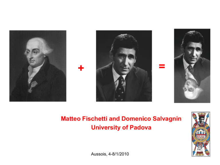
=
+
?
Matteo Fischetti and Domenico Salvagnin
University of Padova
Aussois, 4-8/1/2010
1
Cutting plane methods
•
Cutting plane methods widely used in convex optimization and to provide
bounds for Mixed-Integer Programs (MIPs)
•
Made by two equally important components:
– (i) the separation procedure (oracle) that produces the cut(s) used to
tighten the current relaxation, and
– (ii) the overall search framework that actually uses the generated cuts
and determines the next point to cut
•
In the last 50 years, considerable research effort devoted to the study of (i)
 families of cuts, cut selection criteria, etc.
•
Search component (ii) much less studied by the MIP community  the
standard approach is to always cut an optimal LP vertex
Aussois, 4-8/1/2010
2
The problem
•
Consider a generic MIP:
z(MIP) := min { cT x : x ε X }
and its LP relaxation
z(LP) := min {cT x: x ε P }
P := { x : A x ≤ b },
•
X := { x ε P: xj integer for j ε J }
We are also given a convex set P1 with conv(X) ≤ P1 ≤ P (e.g., the first
GMI closure) described only implicitly through a separation function:
oracle(y) returns a valid linear ineq. for P1 violated by y (if any)
•
We want to (approximately) compute z1 := min {cT x: x ε P1 }
Aussois, 4-8/1/2010
3
Kelley’s cutting plane method
•
A classical search scheme
J. E. Kelley. The cutting plane method for solving convex
programs, Journal of the SIAM, 8:703-712, 1960.
1. Let P’ := { x ε P : x satisfies all cuts generated so far }
2. Find an optimal vertex x* of the current LP: min {cT x: x ε P’ } ,
3. Invoke oracle(x*) and repeat (if a violated cut is found)
•
Practically satisfactory only if the oracle is able to find “deep” cuts
•
Very ineffective in case shallow cuts are generated
•
May induce a dangerous correlation between x* and the returned cut
(e.g. when the cuts are read from the LP tableau)
Aussois, 4-8/1/2010
4
Kelley and Gomory: a problematic
marriage
exponential determinant
growth  unstable system!
LP bound = 5; ILP optimum = 8
Aussois, 4-8/1/2010
5
But… is it all Gomory’s fault?
•
Experiment: take a given LP problem (e.g. root node relaxation of a MIP)
min { cT x: A’ x ≤ b’, A’’ x = b’’, l ≤ x ≤ u }
and define:
– P := { x: A’’ x = b’’, l ≤ x ≤ u }
– constr. list A’ x ≤ b’ can only be accessed through the separation oracle
•
3 cut selection criteria implemented for separation: for a given x* the oracle
returns:
A) the deepest violated cut in the list (Euclidean distance)  “best” facet
B) a convex combination of the deepest one and of the (at most) first 10
violated or tight cuts encountered when scanning the list
C) the cut is first defined as in case B, but then its rhs is weakened so as to
half the degree of violation
Aussois, 4-8/1/2010
6
Output with Kelley’s search (std)
std-A
std-B
std-C
Aussois, 4-8/1/2010
7
But other search schemes work better…
yoyo-A
std-A
yoyo-B
yoyo-C
e.g. yo-yo search…
std-B
std-C
Aussois, 4-8/1/2010
8
Lessons learned
•
Kelley’s method is intrinsically nonrobust
•
Other search methods can survive even with weak cuts (analytic center,
yo-yo search, etc.)
•
As to GMI cuts, reading both the vertex x* to cut and the cuts themselves
from the same tableau soon creates a dangerous feedback (unstable
dynamic system)
•
Kelley + Gomory is problematic in the long run, but … it is not all Gomory’s
fault!
•
In fact, F. and Lodi (2007) report very good bounds by separating
(fractional) Gomory cuts of rank 1 by means of an external MIP solver  a
key ingredient was the new search scheme that decoupled optimization and
separation
•
Results confirmed for GMI cuts by Balas & Saxena and Dash, Gunluk &
Lodi
Aussois, 4-8/1/2010
9
Reading GMIs from LP bases
•
If you insist on reading GMI cuts from an LP basis … at least don’t use an
optimal one!
•
Steps in this direction: given an optimal LP vertex x* of the “large LP”
(original+cuts) and the associated optimal basis B*:
–
Balas and Perregaard (2003): perform a sequence of pivots leading to
a (possibly non-optimal or even infeasible) basis of the large LP
leading to a deeper cut w.r.t. the given x*
–
Dash and Goycoolea (2009): heuristically look for a basis B of the
original LP that is “close to B*” in the hope of cutting the given x* with
rank-1 GMI cuts associated with B
Aussois, 4-8/1/2010
10
Back to Lagrangia
•
Forget about Kelley: optimizing over the first GMI closure reads
min cT x
xεP
< all rank-1 GMI cuts >
•
Dualize (in a Lagrangian way) the GMI cuts, i.e. …
•
… solve a sequence of Lagrangian subproblems
min { c(λ)T x : x ε P }
on the original LP but using the Lagrangian cost vector c(λ)
•
Subgradient s at λ :
si = violation of the i-th GMI cut w.r.t.
x*(λ) := argmin { c(λ)T x : x ε P }
Aussois, 4-8/1/2010
11
Back to Lagrangia
• During the Lagrangian dual optimization process, a large number of
bases of the original LP is traced  round of rank-1 GMI cuts can
easily be generated “on the fly” and stored
• Use of a cut pool to explicitly store the generated cuts, needed to
compute (approx.) subgradients used by Lagrangian optimization
• Warning: new GMI cuts added on the fly  possible convergence
issues due to the imperfect nature of the computed “subgradients”
• … as the separation oracle does not return the list of all violated
GMI cuts, hence the subgradient is truncated somehow …
Aussois, 4-8/1/2010
12
Lagrange + Gomory = LaGromory
•
Generate cuts and immediately dualize them (don’t wait they become wild!)
•
No fractional point x* to cut: separation used to find (approx.) subgrad.s
•
Lagrangian optimization as a stabilization filter in the closed loop system
 GMI cuts are loosely correlated with the underlying large LP (original+
previously generated GMI cuts) as they don’t even see the large tableau
•
The method can add rank-1 GMI cuts on top of nonlinear constraints and of
any other classes of cuts (Cplex cuts etc.), including branching conditions
 just dualize them!
•
Key to success: resist to the “Kelley’s temptation” of reading the GMI
from the optimal tableau of the large LP!
Aussois, 4-8/1/2010
13
Experiments with LaGromory cuts
•
Three preliminary implementations:
– lagr: naïve Held-Karp subgradient opt. scheme (10,000 iter.s)
– hybr: as before, but every 1,000 subgr. iter.s we solve the “large LP”
just to recompute the optimal Lagrangian multipliers for all the cuts in
the current pool
– fast: as before, but faster: only 10 large LPs solved, each followed by
just 50 subgradient iterations with very small step size  10 short walks
around the Lagrangian dual optimum to collect bases of the original LP,
each made by 50 small steps to perturb Lagrangian costs
•
Comparision with std (one round of GMI cuts)
Aussois, 4-8/1/2010
14
Preliminary computational results
Testbed: 32 instances from MIPLIB 3.0 and 2003
CPU seconds on a standard PC (1GB memory allowed)
%gap
Closed
Time
(sec.s)
%gap
closed
Time
(sec.s)
std
24.4%
0.01
std
33.1%
0.02
lagr
63.6%
46.69
lagr
68.9%
72.64
hybr
69.6%
36.97
hybr
73.4%
108.00
fast
59.1%
1.52
fast
69.3%
4.79
Rank 1 GMI cuts
Rank 2 GMI cuts
Aussois, 4-8/1/2010
15
Fast with different parameters
1 walk
5 walks
10 walks 15 walks 20 walks 25 walks
100 steps
per walk
gap
37.00%
56.60%
60.60%
62.00%
62.60%
63.20%
time
0.01
1.26
2.84
4.29
5.71
7.11
50 steps
per walk
gap
36.50%
55.60%
59.10%
61.00%
61.80%
62.40%
time
0.01
0.69
1.52
2.33
3.03
3.72
Rank 1 GMI cuts (std = 24.4% in 0.01 sec.s)
Aussois, 4-8/1/2010
16
… thank you for your attention!
Aussois, 4-8/1/2010
17
Lagrange + Gomory ?
Matteo Fischetti and Domenico Salvagnin
University of Padova
Aussois, 4-8/1/2010
18