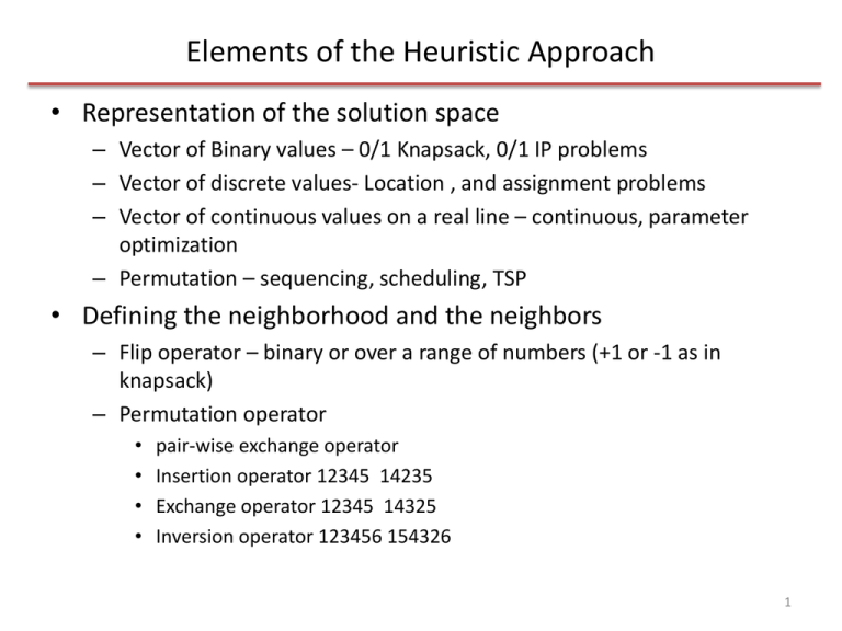
Elements of the Heuristic Approach
• Representation of the solution space
– Vector of Binary values – 0/1 Knapsack, 0/1 IP problems
– Vector of discrete values- Location , and assignment problems
– Vector of continuous values on a real line – continuous, parameter
optimization
– Permutation – sequencing, scheduling, TSP
• Defining the neighborhood and the neighbors
– Flip operator – binary or over a range of numbers (+1 or -1 as in
knapsack)
– Permutation operator
•
•
•
•
pair-wise exchange operator
Insertion operator 12345 14235
Exchange operator 12345 14325
Inversion operator 123456 154326
1
Elements of the Heuristic Approach
• Defining the initial solution
– Random or greedy
• Choosing the method (algorithm for iterative search)
– Off-the shelf or tailor made heuristic
– Single-start or multistart (still single but several independent singles) or
population (solutions interact with one another)
– Strategies for escaping local optima
– Balance diversification and intensification of search
• Objective function evaluation
– Full or partial evaluation
– At every iteration or after a set of iterations
• Stopping criteria
– Number of iterations
– Time
– Counting the number of non-improving solutions in consecutive iterations.
Remember: there is a lot of flexibility in setting up the above. Optimality cannot be proved.
All you are looking for is a good solution given the resource (time, money and computing power)
2
constraints
Escaping local optimas
• Accept nonimproving neighbors
– Tabu search and simulated annealing
• Iterating with different initial solutions
– Multistart local search, greedy randomized adaptive search procedure
(GRASP), iterative local search
• Changing the neighborhood
– Variable neighborhood search
• Changing the objective function or the input to the problem in
a effort to solve the original problem more effectively.
– Guided local search
3
Tabu search – Job-shop Scheduling problems
• Single machine, n jobs, minimize total weighted tardiness, a job
when started must be completed, N-P hard problem, n! solutions
• Completion time Cj
• Due date dj
• Processing time pj
• Weight wj
• Release date rj
• Tardiness Tj = max (Cj-dj, 0)
• Total weighted tardiness = ∑ wj . Tj
• The value of the best schedule is also called aspiration criterion
• Tabu list = list the swaps for a fixed number of previous moves
(usually between 5 and 9 swaps for large problems), too few will
result in cycling and too many may be unduly constrained.
• Tabu tenure of a move= number of iterations for which a move is
forbidden.
4
Problems- Parallel machine flow shop
• m machines and n jobs
– Machines are in parallel, identical and can process all types of jobs
– Ex. 2 machines, 4 jobs
Jobs j
pj
1
9
2
9
3
12
4
3
dj
10
8
5
28
wj
14
12
1
12
Initial solution 3142
Weighted tardiness 163
=7*1+13*12= 163
3
2
12
1
21
4
9
12
5
Problems- Parallel machine flow shop
• m machines and n jobs
– Machines are in parallel, identical and can process all types of jobs
– Ex. 2 machines, 4 jobs
– Each job must flow first on machine 1 then on machine 2
Jobs j
pj
1
9
2
9
3
12
4
3
dj
10
8
5
28
wj
14
12
1
12
Initial solution 3142
Weighted tardiness 881
=19*1+23*14+8*12+37*12
3
1
12
2
21
3
12
4
24
33
1
24
4
33
2
36
45
6
Set-covering problems
• Applications
–
–
–
–
–
–
Airline crew scheduling: Allocate crews to flight segments
Political districting
Airline scheduling
Truck routing
Location of warehouses
Location of a fire station
– Example with Tabu search
7
Simulated Annealing
• Based on material science and physics
• Annealing: For structural strength of objects made from iron,
annealing is a process of heating and then slow cooling to
form a strong crystalline structure.
• The strength depends on the cooling rate
• If the initial temperature is not sufficiently high or the cooling
is too fast then imperfections are obtained
• SA is an analogous process to the annealing process
8
SA
• The objective of SA is to escape local optima and to delay
convergence.
• SA is a memoryless heuristic approach
• Start with an initial solution
• At each iteration obtain a neighbor in a random or organized way
• Moves that improve the solution are always accepted
• Moves that do not improve the solution are accepted using a
probability.
– By the law of thermodynamics at temperature t, the probability of an
increase in energy of magnitude dE is given by
P(dE,t)= exp(-dE/kt)
Where k is the Boltzmann’s constant
For min problems dE = f(current move)-f(last move)
For max problem dE = f(lastmove)- f(current move)
Keep dE positive
9
SA
• The acceptance probability of a non-improving solution is
– P(dE,t) > R
– Where R is a uniform random number between 0 and 1
– Sometimes R can be fixed at 0.5
• At a given temperature many trials can be explored
• As the temperature cools the acceptance probability of a nonimproving solution decreases.
• In solving optimization problems let kt = T
• In summary, other than the standard design parameters such
as neighborhood and initial solution, the two main design
parameters are
– Cooling schedule
– Acceptance probability of non-improving solutions which depends on
the initial temperature
10
SA – acceptance probability of non-improving solutions
•
•
•
•
At high temperature, the acceptance probability is high
When T = ∞ all moves are accepted
When T ~ 0 no non-improving moves are accepted
Note the above decrease in accepting non-improving moves is
exponential.
• Setting initial temperature
– Set very high – accept all moves- high computation cost
– Using standard deviation s of the difference between objective
function values obtained from preliminary experimentation.
• T= cs
– c= -3/ln(p)
– p= acceptance probability
11
SA – Cooling schedules
• Linear
– Ti= T0 – ib where i is the iteration number and b is a constant
• Geometric
– Ti= aTi-1 where a is a constant
• Logarithmic
– Ti= T0/ln(i)
– The cooling rate is very slow but can help to reach global optimum.
Computationally intensive
• Nonmonotonic
– Temp is increased again during the search to encourage diversification.
• Adaptive
– Dynamic cooling schedule. Adjust based on characteristics of the
search landscape
• A large number of iterations at low temp and a small number of iterations
at high temp
12
SA – stopping criteria
• Reaching the final temperature
• Achieving a pre-determined number of iterations
• Keeping a counter on the number of times a certain
percentage of neighbors at each temperature is accepted.
13