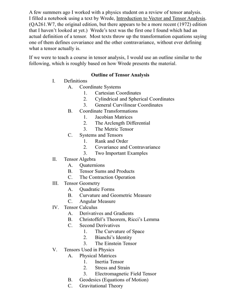
A few summers ago I worked with a physics student on a review of tensor analysis.
I filled a notebook using a text by Wrede, Introduction to Vector and Tensor Analysis.
(QA261.W7, the original edition, but there appears to be a more recent (1972) edition
that I haven’t looked at yet.) Wrede’s text was the first one I found which had an
actual definition of a tensor. Most texts throw up the transformation equations saying
one of them defines covariance and the other contravariance, without ever defining
what a tensor actually is.
If we were to teach a course in tensor analysis, I would use an outline similar to the
following, which is roughly based on how Wrede presents the material.
Outline of Tensor Analysis
I.
Definitions
A. Coordinate Systems
1.
Cartesian Coordinates
2.
Cylindrical and Spherical Coordinates
3.
General Curvilinear Coordinates
B. Coordinate Transformations
1.
Jacobian Matrices
2.
The Arclength Differential
3.
The Metric Tensor
C. Systems and Tensors
1.
Rank and Order
2.
Covariance and Contravariance
3.
Two Important Examples
II. Tensor Algebra
A. Quaternions
B. Tensor Sums and Products
C. The Contraction Operation
III. Tensor Geometry
A. Quadratic Forms
B. Curvature and Geometric Measure
C. Angular Measure
IV. Tensor Calculus
A. Derivatives and Gradients
B. Christoffel’s Theorem, Ricci’s Lemma
C. Second Derivatives
1.
The Curvature of Space
2.
Bianchi’s Identity
3. The Einstein Tensor
V. Tensors Used in Physics
A. Physical Matrices
1.
Inertia Tensor
2.
Stress and Strain
3.
Electromagnetic Field Tensor
B. Geodesics (Equations of Motion)
C. Gravitational Theory
Let n and k be given natural numbers. Any set containing n k elements will be called
a system of order k when the elements are labeled using k indices, with each index used
to label n elements (that is, n k  n  n 
 n is a product of k factors, each of size n.)
For example, vectors can be considered as systems of order 1, and square matrices
represent systems of order 2. Now, a square matrix could also be thought of as a system
of order 1 in which each of the n elements is a row vector. Similarly, a square matrix can
be considered as a sequence of column vectors.
Algebraically, there is no difference between row vectors and column vectors, but because
rows and columns represent the two indices in a system of order 2 we can arbitrarily say
row vectors define one time of system and column vectors define a different type.
 x1 
 
x
We will use subscripts for column vectors, xi   2  , and also refer to these as
 
 
 xn 
covariant vectors. We will use superscripts for row vectors, x j  x1
x2
xn ,
and also refer to these as contravariant vectors. Again, the distinction between these
two terms is completely arbitrary, since algebraically they both represent exactly the
same system.
This last statement is made in terms of vector algebra. If we consider matrix algebra, in
particular matrix multiplication, then there is a difference between row and column vectors.
Considering a row vector as a 1  n matrix and a column vector as an n 1 matrix, the matrix
product is defined when multiplying the vectors in either order, but a row vector times a
column vector gives a 11 result, i.e. a scalar, while a column vector times a row vector
gives an n  n square matrix.
The scalar product between two vectors is also called the inner product between the vectors.
Given a row vector x i and a column vector yi , we define the inner product
 y1 
 
y
x i yi  x1 x 2
x n  2   x1 y1  x 2 y2   x n yn
 
 
 yn 
which (except for the superscript notation) is the usual definition of the vector dot product.
The inner product as defined above also illustrates the notational rule that, if the same letter
is being used as the index in two different locations in an expression, what this means is
that a sum is being formed over that index.
 y1 
 
y
Without repeating the index, the outer product  2  x1
 
 
 yn 
x2
x n is the n  n matrix
with its component in the i th row and j th column given by aij  yi x j . This outer product is
sometimes referred to as the dyadic product of two vectors (other textbooks confusingly
refer to this as "the" tensor product).
Note again the distinction between row and column vectors is arbitrary, and so the inner
product of vectors x and y could also be written as yi x i , since this gives the same sum as
xi yi . Thus, we have that the inner product is a commutative operation, with y i xi  x i yi .
However, the outer product is not commutative. We have instead that yi x j is the transpose
of the matrix defined by xi y j . That is, the transpose of aij is given by a ij .
Let's use binary numerals to illustrate how a given set of numbers can be written as a system
of order 2 in more than one way. Octal numerals use three binary digits, or three bits, and
hexadecimal digits use four bits. Let's consider tetric (two-bit) numerals, which have four
possible numerical values, 0 = 00, 1 = 01, 2 = 10, 3 = 11. Then the 4-vector 0 1 2 3 ,
a system of order 1, can be considered as a system of order 2, where the two pieces of
information are the values (0 or 1) for each of the two digits. We can do this contravariantly,
a ij  00 01 10 11 , with the i blocks distinguished by the value of the first bit, or
 00 
 
10
covariantly, aij    , with the j blocks distinguished by the value of the second bit.
 01 
 11 
 
We can also use these distinguishing traits to define rows and columns in the matrix
 00 01
0
j
j
j
aij  
 . Note if we define bi    and b  0 1 then we have ai  bi b
 10 11 
1
defined in terms of a concatenation outer product.
We could similarly imagine a 2  2  2 array containing the octal digits 000 through 111,
but instead we use multiple subscripts or subscripts to contain the digits in a 4  2 matrix
(take the tetric digits aij and then tack on either a zero or one at the end, giving aijk ), or as
a 2  4 matrix (add a 0 or 1 to the front of a tetric digit a ij ), giving akij , or even as a row
or column 8-vector.
Finally, we could represent hexadecimal digits as a system of order 4, ai1ji12j2 , with the i indices
representing the four components in the 2  2 matrix for the tetric digits, and the j indices
being another copy of this index.
In general, a system of order k can always be represented as a matrix of m by l blocks of
information, with m  l  n k , so that m  n p and l  n q with p  q  k . Next, each of the
"row blocks" can be divided into groups i1 , i2 , , i p (each group containing n components),
and each "column block" is divided into groups j1 , j2 ,
then become components of T  t j11 , 2j2 ,
i ,i ,
, ip
, jq
, jq . The elements of the system
, and T is called a system with covariant valence q
and contravariant valence p. In this setting, another word for system is pseudotensor.
Thus, we are finally able to answer the question, What is a tensor?
Actually, using the notation and definitions of systems from Wrede's text as just
described, we are going to answer the question, "What makes a system a tensor?"
The answer is that if a measurable system T has certain components in a given (fixed)
coordinate system S , and if changing to a new (moving) coordinate system Sˆ changes the
components of T , then there must be some way to calculate the new values tˆ in terms of
the old values t , and that this method of calculation must somehow involve the equations
of transformation for S  Sˆ. When this calculation is performed in a specified way using
xˆ
x
the partial derivatives
(and/or
), then the system T will be referred to as a tensor.
x
xˆ
The manner in which this calculation is specified was described in a previous handout.
In this more general setting, if T  T j11, j22 ,
i ,i ,
, ip
, jq
represents a system of order p  q (with p being
the contravariant valence and q being the covariant valence), then T will be a tensor if,
under a coordinate transformation S  Sˆ , the relation between the components of T and Tˆ
is given by the set of equations T
i1 , i2 ,
j1 , j2 ,
, ip
, jq
x i1

xˆk1
x p xˆ l1

xˆk p x j1
i
xˆ q ˆ k1 , k2 , , k p
Tl , l , , l .
x jq 1 2 q
l
To make this a bit less general, consider a coordinate system S with coordinates x, y, z 
x1 , x 2 , x3 , transformed to a coordinate system Sˆ with coordinates u, v, w  u1 , u 2 , u 3 .
Then a system T jlik of order 4 is a tensor (with covariant and contravariant valence = 2)
if and only if T jlik 
xi x k u s u q ˆ rp
Tsq . Note this expression involves a quadruple sum,
ur u p x j xl
with each sum having three terms (e.g. r  1, 2, 3).
Recall from the previous handout that the gradient of a scalar function is an example of
a covariant vector (a tensor of order 1), while the vector differential is contravariant.
It was also discussed that, using the rules of transformation, a covariant vector gets
transformed into a contravariant vector, and vice versa. Thus, in the above example using
a tensor of order 4, what apparently is really happening is that the contravariant indices i, k
for T become the covariant indices s, q for Tˆ , and the covariant indices j, l for T become
the contravariant indices r , p for Tˆ. If you keep this idea in mind it helps in getting the
correct labels for the indices on the numerators and denominators of the partial derivatives.
Wrede makes the comment that the transformation from Cartesian to spherical coordinates
can be represented as a system of order 3 (the nine partial derivatives relating x, y, z and
 ,  ,  ), but that this system does not represent a tensor. However, the differential dx 
dx, dy, dz does form a tensor, and the columns of the system of order 3 can be used to
define what is called the metric tensor.
Now for a bit of history.
We observe certain quantities, such as the stress and strain existing in the earth's crust,
which have many different components (magnitudes and directions), and these components
keep changing as the earth keeps moving. In trying to describe this situation we have to
keep track of all the different magnitudes and directions, and the concepts and notation of
tensor analysis were created to simplify the study, i.e. so that the equations used in the
calculations could be written in a compact form without having to write down separate
equations for all the different components.
The Irish physicist/mathematician Sir William Hamilton attempted to create such a system
in the 1850's, and following the work of others he developed and published his Theory on
Quaternions in a sequence of papers, August 1854 – April 1855. In particular he was trying
to come up with a way to unify the various vector products between two given vectors x and
y. In terms of more modern notation, there are for example three such vector products:
Inner Product: x  y  x i yi  Scalar (the dot product)
Cross Product:
Outer Product:
 x  y k   ijk xi y j  Vector ("the" vector product)
i
 x  y  j  xi y j  Matrix ("the" tensor product)
We see that each of these products can be written generically as xy  Pxi y j , where P   ij
for the inner product, P   ijk for the cross product, and P  1 for the outer product.
In this way we can see there are many many different kinds of tensor products which can be
defined, each with their own sets of properties.
Now, just as there is no reason to restrict the way in which a vector product may be defined,
there is also no real reason to restrict the number of vectors required to calculate such a
product. For example, in four-dimensional geometry we need to multiply three vectors
at a time in order to create a cross product with properties similar to that for A  B in 3D.
After Hamilton's work and its generalizations people were trying to decide what kinds of
names should be given to the output of these "higher-ordered" vector operations. Apparently,
one early proposal was the term "bivector", but Voigt (1898) pointed out that wasn't a good
choice, because then what term do we use when we raise the order once again? Instead,
Voigt proposed the term "tensor" to include scalars, vectors, matrices, and higher-ordered
algebraic quantities. (The exact reference is given in Wrede's text, which I also used as
inspiration for the following set of notes.)
The word "vector" comes from the Latin root vec- (and from which our word "vehicle"
comes from), meaning to carry something from one place to another. This word was also
used, starting around 1700, to describe an organism which carried a disease from one host
to another. The term was also used in transportation, where piloting a ship across the ocean
began to be referred to as vectoring a course. Thus, scientists in the 18th century began using
the term vector to refer to any quantity that had not only magnitude but also a specified
direction.
Also about this time the word "tensor" (from the Latin verb for "to stretch") was being used
to describe the magnitudes of the various components (e.g. of velocity) pointing in different
directions, with the word "vector" initially referring to just the direction but eventually (as
today) referring to both the magnitude and the direction. Thus, by the end of the 19th century
the word "tensor" wasn't being used much anymore, and so Voigt proposed reviving its use
as referring to the idea (which Voigt originated, according to Wrede) that a tensor specifically
refers to the components describing an object whose measurable components change in a
specified way under a given coordinate transformation.
Today when we wish to refer to magnitude without direction we use the term "scalar".
Since a scalar has no direction, it does not have multiple components, and so its single
measurable value must be the same in all coordinate systems. Since there are zero equations
used to describe a scalar transformation (that is, since a scalar stays the same and does not
transform), a scalar quantity is referred to as a tensor of order zero.
As mentioned earlier, a vector is referred to as a tensor of order one, and the arbitrary
concepts of row vectors vs column vectors is used to motivate the distinction between
covariance and contravariance in describing tensors. I have also tried to show that, even
for tensors of order two, which can be represented as matrices, there really is no difference
between covariance and contravariance, since this just involves writing down the elements
of a set in different orders.
However, when we get to more complicated systems, it will be important to keep track of
covariant and contravariant indices, since changing their roles will result in different answers.
Now, the rules and notation for tensor computations have been developed so that the way to
keep everything in its proper order is basically the way it needs to be in order to obtain a
physically meaningful answer. (This same approach was used by Reynolds in developing
theory for fluid dynamics.)
I will work on future handouts with titles like Tensor Algebra, Tensor Geometry, and
Tensor Calculus, with details about operations such as contraction, the raising and lowering
of indices (transforming contravariance into covariance and vice versa), and how to calculate
derivatives in both a covariant and a contravariant manner. These rules and calculations are
important in being able to reduce the extremely complex problem of gravitational theory to
a single equation. However, for electromagnetic theory we need hardly any of this part of
tensor analysis because electromagnetic fields do not affect the curvature of space to any
magnitude comparable to that of gravitational fields.
Thus, the next thing I will work on this summer is Chapter Three of Landau and Lifshitz's
text, the development of the four-dimensional electromagnetic field tensor.