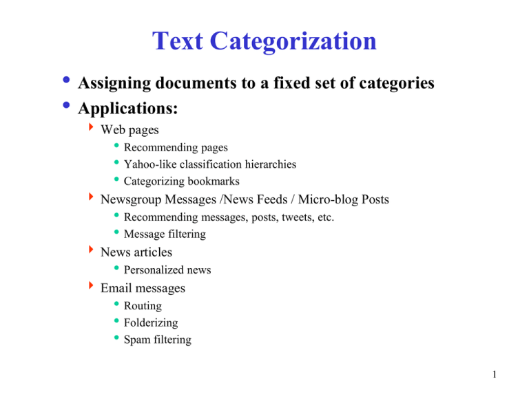
Text Categorization
 Assigning documents to a fixed set of categories
 Applications:
 Web pages
 Recommending pages
 Yahoo-like classification hierarchies
 Categorizing bookmarks
 Newsgroup Messages /News Feeds / Micro-blog Posts
 Recommending messages, posts, tweets, etc.
 Message filtering
 News articles
 Personalized news
 Email messages
 Routing
 Folderizing
 Spam filtering
1
Learning for Text Categorization
 Text Categorization is an application of classification
 Typical Learning Algorithms:
 Bayesian (naïve)
 Neural network
 Relevance Feedback (Rocchio)
 Nearest Neighbor
 Support Vector Machines (SVM)
2
Nearest-Neighbor Learning Algorithm
 Learning is just storing the representations of the
training examples in data set D
 Testing instance x:
 Compute similarity between x and all examples in D
 Assign x the category of the most similar examples in D
 Does not explicitly compute a generalization or
category prototypes (i.e., no “modeling”)
 Also called:
 Case-based
 Memory-based
 Lazy learning
3
K Nearest-Neighbor
 Using only the closest example to determine
categorization is subject to errors due to
 A single atypical example.
 Noise (i.e. error) in the category label of a single training example.
 More robust alternative is to find the k most-similar
examples and return the majority category of these k
examples.
 Value of k is typically odd to avoid ties, 3 and 5 are
most common.
4
Similarity Metrics
 Nearest neighbor method depends on a similarity (or
distance) metric
 Simplest for continuous m-dimensional instance space
is Euclidian distance
 Simplest for m-dimensional binary instance space is
Hamming distance (number of feature values that
differ)
 For text, cosine similarity of TF-IDF weighted vectors
is typically most effective
5
Basic Automatic Text Processing
 Parse documents to recognize structure and meta-data
 e.g. title, date, other fields, html tags, etc.
 Scan for word tokens
 lexical analysis to recognize keywords, numbers, special characters, etc.
 Stopword removal
 common words such as “the”, “and”, “or” which are not semantically
meaningful in a document
 Stem words
 morphological processing to group word variants (e.g., “compute”, “computer”,
“computing”, “computes”, … can be represented by a single stem “comput” in
the index)
 Assign weight to words
 using frequency in documents and across documents
 Store Index
 Stored in a Term-Document Matrix (“inverted index”) which stores each
document as a vector of keyword weights
6
tf x idf Weighs
 tf x idf measure:
 term frequency (tf)
 inverse document frequency (idf) -- a way to deal with the
problems of the Zipf distribution
 Recall the Zipf distribution
 Want to weight terms highly if they are
frequent in relevant documents … BUT
infrequent in the collection as a whole
 Goal: assign a tf x idf weight to each term in each
document
7
tf x idf
wik  tfik * log(N / nk )
Tk  termk in document Di
tf ik  frequencyof termTk in document Di
idfk  inversedocumentfrequencyof termTk in C
N  totalnumber of documentsin thecollectionC
nk  the number of documentsin C thatcontainTk
idfk  log N 
 nk 
8
Inverse Document Frequency
 IDF provides high values for rare words and low values
for common words
 10000
log
0
 10000
 10000
log
  0.301
 5000 
 10000
log
  2.698
 20 
 10000
log
4
 1 
9
tf x idf Example
The initial
Term x Doc matrix
(Inverted Index)
T1
T2
T3
T4
T5
T6
T7
T8
Doc 1
0
1
0
3
0
2
1
0
Doc 2
2
3
1
0
4
7
0
1
Doc 3
4
0
0
1
0
2
0
1
Doc 4
0
0
2
5
0
1
5
0
Doc 5
1
0
0
4
0
3
5
0
Doc 6
0
2
0
0
1
0
1
3
df
3
3
2
4
2
5
4
3
idf = log2(N/df)
1.00
1.00
1.58
0.58
1.58
0.26
0.58
1.00
Documents represented as vectors of words
tf x idf
Term x Doc matrix
T1
T2
T3
T4
T5
T6
T7
T8
Doc 1
0.00
1.58
0.00
1.75
0.00
0.53
0.58
0.00
Doc 2
2.00
0.00
1.58
0.00
6.34
1.84
0.00
1.00
Doc 3
4.00
0.00
0.00
0.58
0.00
0.53
0.00
1.00
Doc 4
0.00
0.00
3.17
2.92
0.00
0.26
2.92
0.00
Doc 5
1.00
0.00
0.00
2.34
0.00
0.79
2.92
0.00
Doc 6
0.00
3.17
0.00
0.00
1.58
0.00
0.58
3.00
10
K Nearest Neighbor for Text
Training:
For each each training example <x, c(x)>  D
Compute the corresponding TF-IDF vector, dx, for document x
Test instance y:
Compute TF-IDF vector d for document y
For each <x, c(x)>  D
Let sx = cosSim(d, dx)
Sort examples, x, in D by decreasing value of sx
Let N be the first k examples in D. (get most similar neighbors)
Return the majority class of examples in N
11