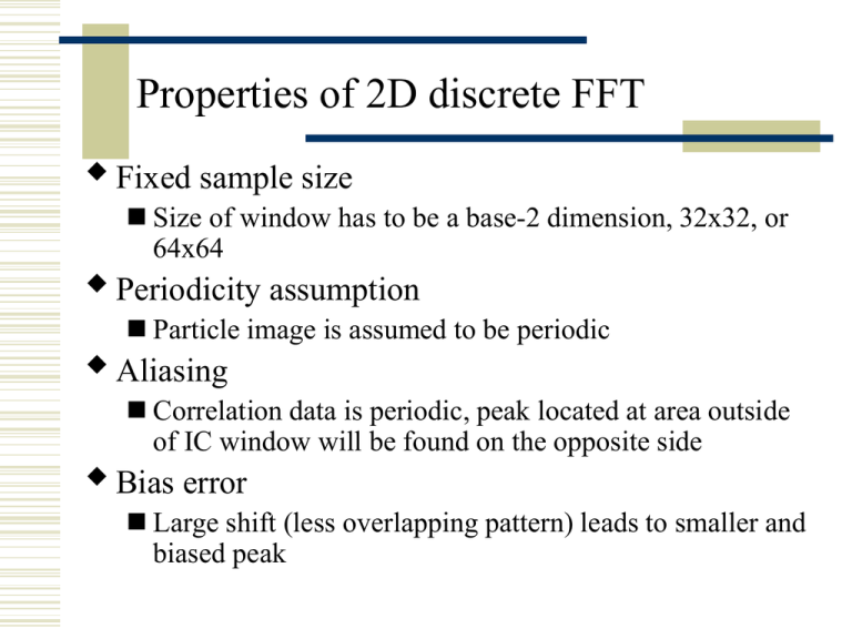
Properties of 2D discrete FFT
 Fixed sample size
 Size of window has to be a base-2 dimension, 32x32, or
64x64
 Periodicity assumption
 Particle image is assumed to be periodic
 Aliasing
 Correlation data is periodic, peak located at area outside
of IC window will be found on the opposite side
 Bias error
 Large shift (less overlapping pattern) leads to smaller and
biased peak
Periodicity assumption
 Applying FFT to a domain assumes the domain is periodic.
Periodicity assumption
 Applying FFT to a domain assumes the domain is periodic.
Periodic condition for the domain
Periodicity assumption
 Applying FFT to a domain assumes the domain is periodic.
Particle image does not
satisfy this condition
Periodic condition for the domain
Periodicity assumption
 Applying FFT to a domain assumes the domain is periodic.
Particle image does not
satisfy this condition
Bias error
Correlation
1
Periodic condition for the domain
Measured
peak
Bias error
True peak
Shift (Ds)
Solution for the bias error
1D example:
1
f
0
1
g
0
Reduce
bias error
0
N
convolving
1
0
0
N
Adjusting
correlation
coefficients
Image is
convolved
with itself
-N/2
N/2
0
Center 0: 1; ±N/2: 1/2
Multiplying
weighting
factors
Re-scale to
[1/2, 1]
Subpixel interpolation
Reason
correlation
correlation
Calculating in
digital form
shift
correlation
Solution: subpixel interpolation
-curve fitting from 3 points near
peak
- finding the peak in the curve
shift
Curve fitting
shift
Schemes for subpixel interpolation
Remark:
-Gaussian fitting is more
commonly used
-Parabolic fitting has a
divided-by-zero problem
when Ri-1 = Ri = Ri+1
Advanced techniques
- multiple pass interrogation algorithm
 Principle
 Crosscorrelating one IC window with another IC window
with known shift
 Determination of known shift – normal crosscorrelation
 Implementation
 Using normal crosscorrelation method to get the velocity
map;
 Detecting bad vectors and replacing with interpolated
vectors;
 Computing crosscorrelation coefficients by shifting
another IC window with the displacement determined by
the obtained velocity;
Advanced techniques
- multiple pass interrogation algorithm
IC
P-II
P-II
P-I
Normal crosscorrelation
P-I
multiple pass interrogation
Advanced techniques
- multiple pass interrogation algorithm
IC
P-II
P-II
P-I
Normal crosscorrelation
P-I
multiple pass interrogation
Advanced techniques
- multiple pass interrogation algorithm
IC
P-II
P-I
Normal crosscorrelation
P-I
P-II
multiple pass interrogation
Advanced techniques
– hierarchical approach
 Principle
 Similar to the multiple pass algorithm but the sampling
grid system is gradually refined with reducing IC size
simultaneously
 Advantage
 Able to capture complex structure;
 Implementation
 Run multiple pass algorithms under adaptive grid
systems and correspondingly changed IC window
Example of hierarchical approach
Multiple peak detection
 Reason
 The strongest peak is not always associated with the
correct shift, especially in the area of complex structure,
e.g., strong vorticity, strong shear
 Implementation
 Detecting local maximums and keeping them as “peak
candidates”;
 Compare velocity with surrounding velocities, ruling out
the unreasonable “peak candidates” until the searching
status is not changed
Example of multiple peak detection
Single peak detection
Multiple peak detection
Data validation
Reason of the occurrence of bad vectors
Inhomogeneous seeding
Noise
Complex flow structure
Validation method
Direct comparison
Median Filter
Mean Filter
Data validation (cont’d)
Direct comparison
U i , j  U i  , j    
 ,   1,1;  0    0
Median Filter
Median (U i , j )  U i , j  
Mean Filter
Mean (U i , j )  U i , j  
U6=Ui-1,j+1
U7=Ui,j+1
U8=Ui+1,j+1
U5=Ui-1,j
U9=Ui,j
U1=Ui+1,j
U4=Ui-1,j-1
U3=Ui,j-1
U2=Ui+1,j-1
Interpolation
Linear interpolation
x3,y3
x4,y4
Dy
x0,y0
x1,y1
Dx
  ( x0  xc ) / 2Dx
1  (1   )(1   ) / 4
3  (1   )(1   ) / 4
U0 
4
 U
i 1
xc,yc
i
i
x1,y1
  ( y0  yc ) / 2Dy
 2  (1   )(1   ) / 4
 4  (1   )(1   ) / 4
Read Tecplot data file
Format of head before data
TITLE = "Import0 in Mae513 Velocity vectors [positions in cm] [velocities in cm/s]"
VARIABLES = " Position x "," Position y "," Velocity u "," Velocity v "
ZONE T="Data", I=34, J=34, F=POINT
DT=( SINGLE, SINGLE, SINGLE, SINGLE )
-3.200000000e+001 -3.200000000e+001 0.000000000e+000 0.000000000e+000
0.000000000e+000 -3.200000000e+001 0.000000000e+000 0.000000000e+000
x
y
u
v
Program list (Matlab)
FileName = 'Take_01000.dat';
%% TecPlot data file which saves velocity data
fid = fopen(FileName,'r');
Line = fgetl( fid ); Line = fgetl( fid ); Line = fgetl( fid );
Dim = sscanf( Line, 'ZONE T="Data", I=%d, J=%d, F=POINT');
Line = fgetl( fid );
nx = Dim(1);
%% Grid number in x direction
ny = Dim(2);
%% Grid number in y direction
u = zeros(nx, ny); v = zeros(nx, ny); x = zeros(nx, 1); y = zeros(1, ny);
temp = fscanf(fid, '%e');
s = 1;
for j = 1:ny
for i = 1:nx
x(i, 1) = temp(s); y(1, j) = temp(s+1); u(i,j) = temp(s+2);
v(i,j) = temp(s+3); s = s + 4;
end
end
fclose(fid);
%% now you have x(1:nx, 1), y(1, 1:ny), u(1:nx, 1:ny), v(1:nx,1:ny)
%% you can do further processing of x, y, u, v
Program list (Fortran)
!! maximum dimension for u and v
parameter (mx = 101, my = 101)
real x(mx), y(my), u(mx,my), v(mx,my)
character*32 FileName /'Take_01000.dat'/
character*80 Line
open(100, file=FileName, status = 'old')
read(100, *); read(100, *); read(100, '(A80)') Line; read(100, *)
!! The line contains the string of
!! 'ZONE T="Data", I=%d, J=%d, F=POINT'
ie1 = index(Line, 'I=') + 2
ie2 = index(Line, ', J=') - 1
ie3 = index(Line, 'J=') + 2
ie4 = index(Line, ', F=POINT') - 1
read(Line(ie1:ie2), '(I)') nx
read(Line(ie3:ie4), '(I)') ny
do j=1, ny
do i=1, nx
read(100, *) x(i), y(j), u(i,j), v(i,j)
enddo
enddo
close(100)
Program list (C/C++)
#include <stdio.h>
#include <stdlib.h>
// maximum dimension for x and y directions
#define MX
101
#define MY
101
int main() {
char FileName[32]; int nx, ny; char Line[81];
float x[MX], y[MY], u[MY][MX], v[MY][MX];
strcpy(FileName, "Take_01000.dat");
FILE *fp = fopen(FileName, "r"); if ( !fp ) return -1;
fgets(Line, 80, fp); fgets(Line, 80, fp); fgets(Line, 80, fp);
fgets(Line, 80, fp); // printf("%s", Line);
sscanf(Line, "ZONE T=\"Data\", I=%d, J=%d, F=POINT\n", &nx, &ny);
printf("nx=%d ny=%d\n", nx, ny);
fgets(Line, 80, fp);
for (int j=0; j<ny; j++)
for (int i=0; i<nx; i++) {
fscanf(fp, "%e %e %e %e", &x[i], &y[j], &u[j][i], &v[j][i]);
}
fclose(fp);
}