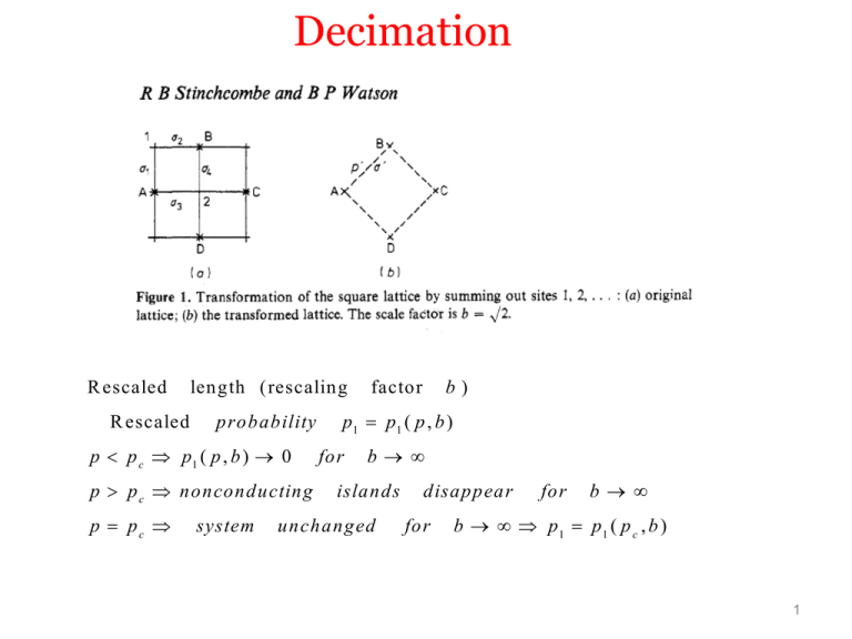
Decimation
R escaled
R escaled
length (rescaling
probability
p  p c  p1 ( p , b )  0
p  p c  nonconducting
p  pc 
system
factor
b)
p1  p1 ( p , b )
for
b 
islands
unchanged
disappear
for
for
b 
b    p1  p1 ( p c , b )
1
To
proceed find a
simple approximation
to p1  p1 ( p , b )
Consider only paths involving a,b,c,d.
What is the probability p1 that nodes A and B of new lattice are connected?
1
B
b
a

d
A
C
2
D
L et
P (a , b ,  , d )  probability
P (a , b ,  )  probability
that
a , b , ,d
that
are
connected,
α ,β ,γ are conected bu t δ is not,
and
so
on.
p 1  P (a , b ,  , d )  P ( a , b ,  )  P ( a , b , d )  P ( a ,  , d )  P ( b ,  , d )  P ( a , b )  P (  , d )
renorm al izati on of p :
p1  p  4 p (1  p )  2 p (1  p )  2 p  p
4
3
2
2
2
4
2
R enorm aliza tion
of
bond
 d p1  4 p (1  p )d p   
2
at
each
scaling
p1  2 p  p
2
4
p
d p1
dp
changes
 Fixed
p1  2 p  p
2
probability :
point
4
 4 p (1  p )
2
by
a
f actor
 ( p ).
equation:
pc  2 pc  pc
2
4
pc  0
T rivial
Fixed
point : repeated
scaling  no
pc  1
T rivial
Fixed
point : repeated
scaling  perfec t
p c   1.6
nonsense
nontrivial
fixed
solution :
cond uctance
conductance
point
p c  0.618
(E xact
result
p c  0.5)
3
A t fixed point:
E xact
 c   ( p c )  1.528 (using p c  0.618) w hile p c  0 .5 yields 1.5.
p c  0.5 and at fix ed p oint:
results know n :
R escaled
length (rescaling
factor
 ( pc )  c 
3
2
b ),
1
the correl ation
b
2

length
  0. 818
E m pirical
Z pc 
i ndex
law
d
d 1

is defined
( exact  
for
various
ln( b )
ln(  )

lattices
b  c
by
ln( 2 )
3
 0.8547 ).
ln ( )
2
in
dim ensio ns
d  2, 3 :
, Z  coordination num ber= num ber of nearest neighbors.
S quare lattice: d= 2, Z= 4, p c = 0.5.
4
Onset of conductivity (R. Rosman-B. Shapiro Phys. Rev. B16, 5117 (1977))
C onductance of netw ork   0
   * ( p  pc ) ,
t
(generalized
for
p  pc

at conductance threshold: p  p c
M ac
1
L aurin;
this defines the coefficient  * and the critical exponent t).
H ow
to
evaluate
t
?
conductance  is
Principle:
To
get
t
us e
scale
invariant
B
b
 ( p ,  )   ( p1 ,  1 )   * ( p  p c )   1 * ( p1  p c )
t
P ath conductances:
a
A
p  pC
condition on s calin g :
t
1
at

d
2
conductance of the series of tw o conductances 
C
1

2
D
conductance of tw o conductances  in parallel
2
5
Evaluation of conductance 1 of
renormalized bond AB
p1 1 

p ( path ) ( path )
1
B
b
a

d
A
(w eighted average)
C
2
paths
probability
of
both
paths
D
a b and d = p ,
4
conductance of com bination of both paths :  ( path )  2
1

2
probability
of
path
through
probability
of
no
path
probabil ity
of
path
through
2
1:
p ,
2: 1 p
through
1
and
conductance of path through 1 onl y :
no
2
path
 ( p ath ) 
1
through
2:
p (1  p )
2
2

2
p1 1  w eighted average  p .2.
4
For
1
2
1
  2 p .(1  p ) .   p  .
2
2
2
2
p  p c , renorm alized p1  p c ,  p c 1  p  
2
c
1

 pc
6
Evaluation
to
get
t
of critical exponent t
use scale invariance conditi o n
1
 ( p ,  )   ( p1 ,  1 )
  * ( p  p c )   1 * ( p1  p c )
t
a
t
 (d p )   1 (d p1 ) 
R ecall:
t
1

 pc

t ln(
d p1
t ln(
R ecall the renorm alization
d p
d p1
d p
Using th is,
1
)  ln(
1
d
2
C
D
).
).
pc
of
 d p1  4 p (1  p )d p   
2
)  ln(


A
 for a sm all increm ent of bond conductivity,
t
B
b
bond
d p1
d p
probabil ity :
p1  2 p  p
2
4
 4 p (1  p ).
 ( p c )   c  1.528
2
and p c  0.61 8
W e get the estim ate t  1.134.
   * ( p  p c ) . A n increase of p near the critical point yields a
t
m ore than proportional grow th of  .
7
Renormalization group for the 1d Ising model
H    J s n s n 1
Z  Tre
b H
F   K B T log Z .
n
Z 

exp[ K ( s 0 s1  s1 s 2  s 2 s 3  s 3 s 4 
)],
K 

exp[ K ( s1 s 2  s 2 s 3 )] exp[ K ( s 3 s 4  s 4 s 5 )]
,
K BT
{ s}
Z 
J


 
{ s}
i
si  
,
{ s}
1
2
3
4
Decimation Eliminating even sites: we must sum over even sites.
Sum over spin 2:

exp[ K ( s1 s 2  s 2 s 3 )]  exp[ K ( s1  s 3 )]  exp[  K ( s1  s 3 )]
s2  
Sum over all even sites:
 
s2  
exp[ K ( s1 s 2  s 2 s 3 )] exp[ K ( s 3 s 4  s 4 s 5 )]

s4  
[exp[ K ( s1  s 3 )]  exp[  K ( s1  s 3 )]][exp[ K ( s 3  s 5 )]  exp[  K ( s 3  s 5 )]
8
Decimation Eliminating even sites: we must sum over even sites AND set
the result back in the original form (as far as we can).
 
O riginal:
s2  
decim ation:
exp[ K ( s1 s 2  s 2 s 3 )] exp[ K ( s 3 s 4  s 4 s 5 )]
K 
K BT
s4  
exp[ K ( s1 s 2  s 2 s 3 )]  e
K ( s1  s 3 )
e
 K ( s1  s 3 )
J
. R esult
s2
m ust
be
W e w ant that if s1
e
K ( s1  s 3 )
If s1
e
 A( K )e
rew ritten
e
 K ( s1  s 3 )
and
s3
K ( s1  s 3 )
e
b ( k ) s1 s 3
(1)
 b(K ) 
A ( K ), b ( K ) .
 2 cosh(2 K )  W e require 2 cosh (2 K )  A ( K ) e
have
 K ( s1  s 3 )
1
appropr iate
s 3 are both  1 or both   1 :
and
opposite
b(k )
signs :
 2  W e require 2  A ( K ) e
 2 cosh(2 K )  A ( K ) e b ( k )

b(k )
2

A
(
K
)
e

K
w ith
b(k )
M ultiplying :
di vi ding :
.
A ( K )  2 cosh( 2 K )
c os h( 2 K )  e
2b(k )
ln cosh( 2 K )
2
Z (K , N ) 
N

{ odd
A ( K )e
s}
b ( k ) s1 s 3
A ( K )e
b ( k ) s3 s5
 A(K ) 2 Z (K
( 1)
,
N
),
2
9
Fixed point:
K 
1
ln cosh(2 K )
 K 0
2
no ferromagnetism, no phase transition, no long-range order!
Renormalization group for the 2d Ising model
(see Grosso-Pastori,McComb)
Z 

{ s}
exp[ K ( s 0 s1  s 0 s 2  s 0 s 3  s 0 s 4 )] exp[ K ( s 5 s1  s 5 s 4  s 5 s 9  s 5 s10 )]
K 
J
K BT
Eliminate site 0

e
K ( s 0 s1  s 0 s 2  s 0 s 3  s 0 s 4 )
e
K ( s1  s 2  s 3  s 4 )
e
 K ( s1  s 2  s3  s 4 )
s0
2 cosh(4 K ) all up + all dow n


  2 cosh(2 K ) three up/dow n and one dow n/up (4 w ays)

2 tw o up and tw o dow n (6 w ays)

New couplings are needed to represent all possibilities:

exp[ K ( s 0 s1  s 0 s 2  s 0 s 3  s 0 s 4 )]  exp[ K ( s1  s 2  s 3  s 4 )]  exp[  K ( s1  s 2  s 3  s 4 )]
s0
 A ( K ) exp [ b ( K )( s1 s 2  s 2 s 3  s 3 s 4  s 4 s1  s1 s 3  s 2 s 4 )] ex p[ c ( K ) s1 s 2 s 3 s 4 ]
Indeed we can fix the uknowns by solving the 16 equations that arise from the
possible spin orientations and that we can summarize in three cases:

exp[ K ( s 0 s1  s 0 s 2  s 0 s 3  s 0 s 4 )]  exp[ K ( s1  s 2  s 3  s 4 )]  exp[  K ( s1  s 2  s 3  s 4 )]
s0
 A ( K ) exp[ b ( K )( s1 s 2  s 2 s 3  s 3 s 4  s 4 s1  s1 s 3  s 2 s 4 )] exp[ c ( K ) s1 s 2 s 3 s 4 ]
2 cosh(4 K )
all up or all dow n  A ( K ) exp[6 b  c ]


  2 cosh(2 K )
three up / dow n and tw o do w n / up  A ( K ) exp[  c ]

2
tw o up and tw o dow n  A ( K ) exp[  2 b  c ]

1
1
A ( K )  2 co sh (2 K ) 2 co sh (4 K ) 8
b(K ) 
1
ln co sh (4 K )
8
c(K ) 
1
8
ln co sh (4 K ) 
1
ln co sh (2 K )
2
12
Iterating,
Z 

exp[ K ( s 0 s1  s 0 s 2  s 0 s 3  s 0 s 4 )] exp[ K ( s 5 s1  s 5 s 4  s 5 s 9  s 5 s10 )]
{ s}
N
 Z  A ( K ) T re
2
(1)
H
(1 )
A ( K )  2 cosh(2 K ) cosh(4 K ) 8
2
  2 b ( K )  si s j  b ( K )  si s j  c ( K )  si s j s k sl
i, j

1
1
H
neareast
i, j
[i, j ]
n eighbours ,  next
i, j
neareast
neighbour s
[i, j ]
This is unlike the original H and interations bring interactions of
increasing complexity. Approximations needed.
N eglect of red and blue term s :
b(K ) 
1
ln cosh(4 K )  K  iteration
lea d s
to
K 0
8
no ferromagnetism, no phase transition, no long-range order!
13
H
(1)
  2 b ( K )  si s j  b ( K )  si s j  c ( K )  si s j s k sl
i, j

neareast
[i, j ]
n eighbours ,  next
i, j
i, j
neareast
neighbour s
[i, j ]
H.J. Maris-L.P.Kadanoff,am.J.Phys.46, 652 (1978):
N eglect of red and blue term s but reinfo rced b(K )
b(K ) 
3
ln cosh(4 K )  iteration
leads
to
K
8
T he solution of K * 

3
ln cosh(4 K
(i)
)
8
3
8
ln cosh(4 K *) is K  K c  0.507.
P rediction: phase transition at K c  0.507
K  K c  0.507
( i  1)
is the nontrivial
fixed
( K O nsager  0.441)
po int
14
Peierls transition in 1d chains
regular 1d chain
a
a
a
Consider a 1d chain of identical equally spaced atoms at hal filling. Peierls in the thirties has shown that in the BornOppenheimer approximation the system is unstable and the ground state shows alternating long and short bond lengths.
Peierls distorted 1d chain
a+u
a-u
The lattice parameter doubles, the BZ becomes the half and a gap opens.This is called a charge density wave (CDW)
state, which can be seen in X-Ray diffraction. All the occupied states go down in energy..
2
T he cost in strain energy goes w ith u ; o ne finds that for sm all displacem ents u
u
2
the gain in kinetic energy goes like u ln ( ).T his is w hy the regular chain is pred icted
a
to be unstable
Polyacetylene with its anternating singe and double bond is the most
common example of the Peierls distortion. Often 1d systems are poor
models of 3d crystals because there are qualitative differences.
See e.g. Sander van Smaalen, Acta Crystallographica (2005)
Jordan-Wigner string
In 1d one can make Fermions out of Bosons
Consider a boson field is defined on a chain, with annihilation
†
operators ci [ c , c ]  0  [ c † , c † ]
[c , c ]  d
i
j

i
j

i

j
ij
How can we use them to define anticomuting fermions? In fact, we can in 1d. The
fermions are:
 i  n
 i  c c
i  n
†
j
j
fi  e
ci  e
ji
j
ji
j
†
fi  e
ci
ji
†
ci
w ith  i  n j called the Jordan-W igner string.
ji
T he key observation is that s inc e e
†
ca e
e
i n a
†
ca e
e
i n a
i n a
†
n a  even  c a n a  even 
†
c a n a  eve n  e
i n a
i n a
 1, e
i odd
  1,
na  1 na  1
n a  1 n a  odd   n a  1 n a  1
†
n a  odd   c a n a  odd   n a  1 n a  1
†
c a n a  odd  e
 ca e
i n a
 ca e
 i n a
†
i even
e
i n a
e
†
Instead, c a
†
i n a
na  1 na  1 
na  1 na  1
†
c a  0 , that is, c a anticom m utes w ith e
 i n a
and
c a  0 but also c a e
ca
i n a
com m ute w ith
e
e
i n a
i n b
in a
.
ca .
for a  b.
18
18
†
a
i
†
a
f f
i
e
 nj
ja
 nj
i
†
a
jb
c e
†
†
b
†
†
cb  c a e
i ( n a  n a  1 
 n b 1 )
†
c b since w e can
 nj
j a
chop e
†
b
†
fa fb  fb fa  0
So, we can verify that in the following situation,
on sites on left of site a, nam ely a-1,a-2,... since they occur tw ice;
†
†
one can also w rite: f a f b  e
i ( n a  1 
 n b 1 )
†
ca e
i n a
†
cb
(com m utatio n on different sites)
i
†
b
O n th e o th er h an d , f f
†
a
e
 nj
jb
i
†
b
 nj
ja
c e
†
†
d eletin g th o se o ccu rrin g tw ice, f b f a  e
†
†
†
†
e
i n a
S o, fa fb  fb fa =
†
sin ce c a e
i n a
e
i ( n a  1 
†
[ca e
i n a
i ( n a  n a  1 
e
i n a
†
 n b 1 )
†
†
cb c a .
†
c a ]c b  0
†
ca  0.
 i
T hus,
 n b 1 )
†
ca ;
fi  e
 nj
ji
 i
ci  e
 c jc j
†
ji
c i is a Ferm ion.
x
There is also a continuous version
 i
f ( x)  e
 dx '  ( x ')

c ( x ).
Jordan-Wigner string with Pauli matrices 
x
y z
Let us associate Pauli matrices to sites of a chain. Matrices of different sites
commute. Then introduce the matrices
i
Cm  e
  j j



m,
j m
i
W e can w rite C m  e
  j j

jm
i



m
†
0

1 m
T herefore, C m   m  (  n )

z
1

 i
0
e
0

0 n
nm



j m
m
0

0
0

1 m
 Cm  e
0

0
  j j
 e i
 0
nm 
0

1 n
C m   m  (  n ).
†
È
nm

z
nm
They anticommute and are Fermion annihilation and creation operators
Indeed the Jordan-Wigner factors can be removed when they occur twice, so on site
1
[ C m , C ]   (  (  )) [ ,  ]   [ ,  ]   [ 
nm
0
†
m
z
n


 C m C m   m m .
†
2

m

m

m

m
0 0
,
0 1
0
 ]   1.
0
20
O ff  site, anti com m utatio n
is also obtained:
†
for instance let's w ork out [ C 4 , C 2 ]  .
W e m ay start the Jordan-W igner stri ng C m   m  (  n ) from j= 1

z
nm

C 4  (  1 )(  2 )(  3 ) 4
†
z
z
z

C 2  (  1 ) 2 .
z




[ C 4 , C 2 ]   (  1 ) (  2 ) (  3 ) 4  (  1 ) 2  (  1 ) 2  (  1 ) (  2 ) (  3 ) 4
†
z
z
z
z
z
z
z
z
and elim inating the square of  1 w e are left w i t h
z




[ C 4 , C 2 ]   ( 2 )( 3 ) 4  2   2 ( 2 ) ( 3 ) 4
†
z
z


z
[ C 4 , C 2 ]   [ 2 ,  2 ]   3  4  0 since
†
z
z
z

[ ,  ]   0.
z
21
The Onsager solution of the 2d Ising model

H Ising  
J si s j   H
s
j
adjacent i , j
on N xN square lattice
H  0 otherw ise no solution.
The partition function is:
Z e
b FN
2

 

s1 ,1   s1 ,2  

e
 b H Ising
s N ,N  
site notation:
Notation:
.
K  bJ
s i is specified as s row , colum n .
The geometry of a torus is adopted, identifying column N+1 with column 1
and row N+1 with row 1, that is, imposing pbc
s n , N 1  s n ,1 ,
s N 1, m =s 1, m .
22
First step: write Z in terms of the eigenvalues of a Hermitean matrixthe transfer matrix V. This will be chosen with the structure of a onedimensional
array.
23
Row-by-row description
Let  a  { sa ,1 , sa , 2 , sa ,3 ,  , sa , N } denote a configuration of the spins in the row a ;
there are 2
N
configurations for each ro w . T he set {  a , a  1,
assigns one of the 2
Z 
N
N}
2
 
configurations of the lat tic e.

s1 ,1   s1 ,2  

sN ,N  
e
 b H Ising

 e
1
2
 b H Ising
.
N
Indeed, in the l.h.s. we are summing on all the configurations taking them site by
site, in the r.h.s. we do the same thing row by row.
H ow ever w e have to w rite
e
 b H Ising
in a suitable w ay for a row  by  row description.
24
Z 
 


s1 ,1   s1 ,2  
e
 b H Ising

 e
1
sN ,N  
2
 b H Ising
.
N
N
T he interaction energy betw een the spins w ithin row a is
E (  a )   J  sa , k sa , k  1
k
N
B esides, interaction energy betw een adj acent row s:
E (  a ,  a  1 )   J  sa , k sa  1, k
k 1
For each lattice configuration Z has a contribution
e
 b E ( 1 )  b E ( 1 ,  2 )
e
 b E ( 2 ) b E (  2 ,3 )
e
 b E (  N )  b E (  N , 1 )
.
D efine for each row the N -dim ension al m ultiindex
 a  { sa ,1 , sa , 2 , sa ,3 ,  , sa , N }
that can take 2
N
  a | V |  a 1   e
H e nc e ,
N
values, and the 2 X 2
 b E (  a )  b E (  a ,  a 1 )
  a | V |  a 1   e
N
T ransfer m atrix :
,
 b E (  a )  b E (  a ,  a 1 )
N


k
e
b Jsa , k sa , k 1
e
b Jsa , k sa 1 , k
.
25
Example:N=3
 1  ( s1 1 , s 1 2 , s 1 3 )
T he system has 2  512 configurations
9
 2  ( s 21 , s 22 , s 23 )
Z= 
 3  ( s31 , s32 , s33 )
 1 | V |  2   e
1
 b E ( 1 )  b E ( 1 ,  2 )
 
2
3


e
e
bH
3
b Js1 , k s1 , k 1
e
b Js1 , k s 2 , k
3
is 2 X 2
3
k
since  1 depends on 3 spins,  2 depends on 3 spins.
For each lattice configuration Z has a contribution
e
Z 
 b E ( 1 )  b E ( 1 ,  2 )
   
1
2
N
1
e
 b E ( 2 ) b E ( 2 ,3 )
e
 b E (  3 )  b E (  3 , 1 )
| V |  2   2 | V |  3    2 | V |  1  
 
.
| V |  1   T rV
3
1
1
is w ritten in term s of a 8X 8 m atrix. W e can do the sam e in gene ra l .
3