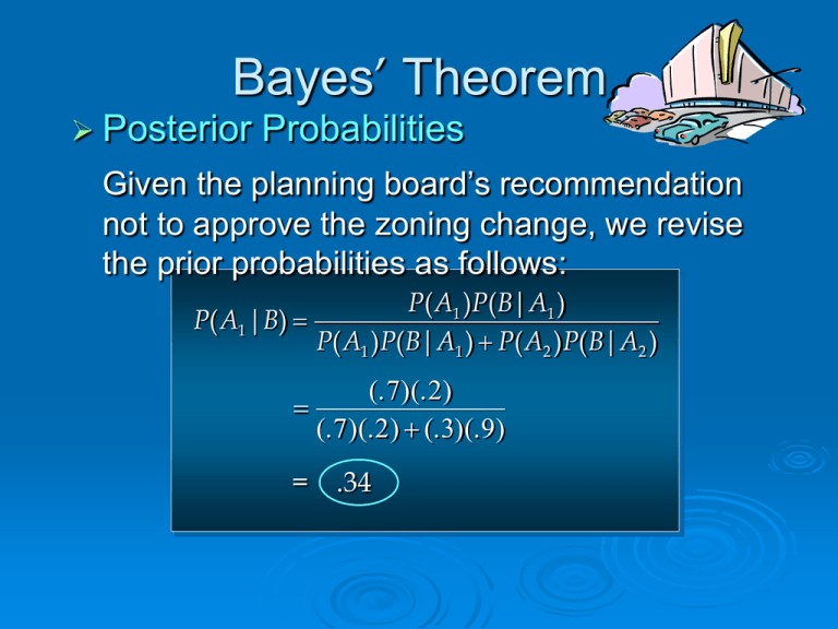
Bayes’ Theorem
 Posterior
Probabilities
Given the planning board’s recommendation
not to approve the zoning change, we revise
the prior probabilities as follows:
P( A1 )P( B| A1 )
P( A1 |B) 
P( A1 )P( B| A1 )  P( A2 )P( B| A2 )
(. 7)(. 2)

(. 7)(. 2)  (.3)(.9)
= .34
Bayes’ Theorem

Conclusion
The planning board’s recommendation is good news
for L. S. Clothiers. The posterior probability of the town
council approving the zoning change is .34 compared to a
prior probability of .70.
Tabular Approach
 Step
1
Column 1 the
- Thefollowing
mutually exclusive
for which
Prepare
threeevents
columns:
posterior probabilities are desired.
Column 2 - The prior probabilities for the events.
Column 3 - The conditional probabilities of the new
information given each event.
Tabular Approach
(1)
(2)
(3)
Prior
Conditional
Events Probabilities Probabilities
Ai
P(Ai)
P(B|Ai)
A1
A2
.7
.3
1.0
.2
.9
(4)
(5)
Tabular Approach
 Step
2
Column 4
Compute the joint probabilities for
each event and the new information B by
using the multiplication law.
Multiply the prior probabilities in
column 2 by the corresponding conditional
probabilities in column 3. That is, P(Ai IB)
= P(Ai) P(B|Ai).
Tabular Approach
(1)
(2)
(3)
(4)
Prior
Conditional
Joint
Events Probabilities Probabilities Probabilities
Ai
P(Ai)
P(B|Ai)
P(Ai I B)
A1
A2
.7
.3
1.0
.2
.9
(5)
.14
.27
.7 x .2
Tabular Approach

Step 2 (continued)
We see that there is a .14 probability of the town
council approving the zoning change and a negative
recommendation by the planning board.
There is a .27 probability of the town council
disapproving the zoning change and a negative
recommendation by the planning board.
Tabular Approach
Column 4
 Step
3
Sum the joint probabilities. The sum is the
probability of the new information, P(B). The sum
.14 + .27 shows an overall probability of .41 of a
negative recommendation by the planning board.
Tabular Approach
(1)
(2)
(3)
(4)
Prior
Conditional
Joint
Events Probabilities Probabilities Probabilities
Ai
P(Ai)
P(B|Ai)
P(Ai I B)
A1
A2
.7
.3
1.0
.2
.9
.14
.27
P(B) = .41
(5)
Tabular Approach
 Step
4
Column 5
Compute the posterior probabilities
using the basic relationship of conditional
probability. P( A | B)  P( Ai  B)
i
P( B)
The joint probabilities P(Ai I B) are in
column 4 and the probability P(B) is the
Tabular Approach
(1)
(2)
(3)
(4)
(5)
Prior
Posterior
Conditional
Joint
Events Probabilities Probabilities Probabilities Probabilities
Ai
P(Ai)
P(Ai |B)
P(B|Ai)
P(Ai I B)
A1
A2
.7
.3
1.0
.2
.9
.14
.27
P(B) = .41
.14/.41
.3415
.6585
1.0000
Homework
 P142-2
P
143-6,9,10
 P146-15,17
 P152-23
 P153-28
 P158-30,33
 P165-39,42
End of Chapter 4