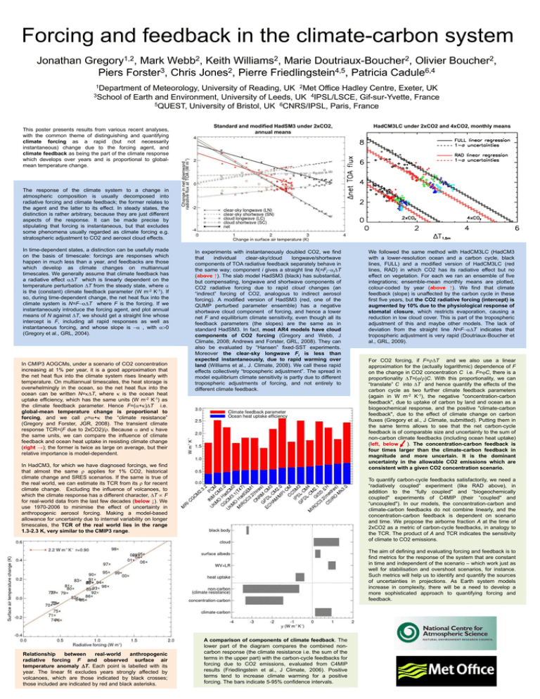
Forcing and feedback in the climate-carbon system
Jonathan
1,2
Gregory ,
2
Webb ,
2
Williams ,
2
Doutriaux-Boucher ,
Mark
Keith
Marie
Olivier
3
2
4,5
6,4
Piers Forster , Chris Jones , Pierre Friedlingstein , Patricia Cadule
2
Boucher ,
1Department
of Meteorology, University of Reading, UK 2Met Office Hadley Centre, Exeter, UK
3School of Earth and Environment, University of Leeds, UK 4IPSL/LSCE, Gif-sur-Yvette, France
5QUEST, University of Bristol, UK 6CNRS/IPSL, Paris, France
This poster presents results from various recent analyses,
with the common theme of distinguishing and quantifying
climate forcing as a rapid (but not necessarily
instantaneous) change due to the forcing agent, and
climate feedback as being the part of the climate response
which develops over years and is proportional to globalmean temperature change.
Standard and modified HadSM3 under 2xCO2,
annual means
HadCM3LC under 2xCO2 and 4xCO2, monthly means
The response of the climate system to a change in
atmospheric composition is usually decomposed into
radiative forcing and climate feedback; the former relates to
the agent and the latter to its effect. In steady states, the
distinction is rather arbitrary, because they are just different
aspects of the response. It can be made precise by
stipulating that forcing is instantaneous, but that excludes
some phenomena usually regarded as climate forcing e.g.
stratospheric adjustment to CO2 and aerosol cloud effects.
In time-dependent states, a distinction can be usefully made
on the basis of timescale: forcings are responses which
happen in much less than a year, and feedbacks are those
which develop as climate changes on multiannual
timescales. We generally assume that climate feedback has
a radiative effect T which is linearly dependent on the
temperature perturbation T from the steady state, where 
is the (constant) climate feedback parameter (W m-2 K-1). If
so, during time-dependent change, the net heat flux into the
climate system is N=FT where F is the forcing. If we
instantaneously introduce the forcing agent, and plot annual
means of N against T, we should get a straight line whose
intercept is F, including all rapid responses as well as
instantaneous forcing, and whose slope is  , with 0
(Gregory et al., GRL, 2004).
In CMIP3 AOGCMs, under a scenario of CO2 concentration
increasing at 1% per year, it is a good approximation that
the net heat flux into the climate system rises linearly with
temperature. On multiannual timescales, the heat storage is
overwhelmingly in the ocean, so the net heat flux into the
ocean can be written N=T, where  is the ocean heat
uptake efficiency, which has the same units (W m-2 K-1) as
the climate feedback parameter. Hence F=(+)T i.e.
global-mean temperature change is proportional to
forcing, and we call =+ the “climate resistance”
(Gregory and Forster, JGR, 2008). The transient climate
response TCR=(F due to 2xCO2)/. Because  and  have
the same units, we can compare the influence of climate
feedback and ocean heat uptake in resisting climate change
(right →); the former is twice as large on average, but their
relative importance is model-dependent.
In experiments with instantaneously doubled CO2, we find
that
individual
clear-sky/cloud
longwave/shortwave
components of TOA radiative feedback separately behave in
the same way; component i gives a straight line Ni=FiiT
(above ↑). The slab model HadSM3 (black) has substantial,
but compensating, longwave and shortwave components of
CO2 radiative forcing due to rapid cloud changes (an
“indirect” forcing of CO2, analogous to indirect aerosol
forcing). A modified version of HadSM3 (red, one of the
QUMP perturbed parameter ensemble) has a negative
shortwave cloud component of forcing, and hence a lower
net F and equilibrium climate sensitivity, even though all its
feedback parameters (the slopes) are the same as in
standard HadSM3. In fact, most AR4 models have cloud
components of CO2 forcing (Gregory and Webb, J
Climate, 2008; Andrews and Forster, GRL, 2008). They can
also be evaluated by “Hansen” fixed-SST experiments.
Moreover the clear-sky longwave Fi is less than
expected instantaneously, due to rapid warming over
land (Williams et al., J. Climate, 2008). We call these rapid
effects collectively “tropospheric adjustment”. The spread in
model equilibrium climate sensitivity is partly due to different
tropospheric adjustments of forcing, and not entirely to
different climate feedback.
In HadCM3, for which we have diagnosed forcings, we find
that almost the same  applies for 1% CO2, historical
climate change and SRES scenarios. If the same is true of
the real world, we can estimate its TCR from its  for recent
climate change. Excluding the influence of volcanoes, to
which the climate response has a different character, T  F
for real-world data from the last few decades (below ↓). We
use 1970-2006 to minimise the effect of uncertainty in
anthropogenic aerosol forcing. Making a model-based
allowance for uncertainty due to internal variability on longer
timescales, the TCR of the real world lies in the range
1.3-2.3 K, very similar to the CMIP3 range.
We followed the same method with HadCM3LC (HadCM3
with a lower-resolution ocean and a carbon cycle, black
lines, FULL) and a modified version of HadCM3LC (red
lines, RAD) in which CO2 has its radiative effect but no
effect on vegetation. For each we ran an ensemble of five
integrations; ensemble-mean monthly means are plotted,
colour-coded by year (above ↑). We find that climate
feedback (slope) is unaffected by the carbon cycle in these
first five years, but the CO2 radiative forcing (intercept) is
augmented by 10% due to the physiological response of
stomatal closure, which restricts evaporation, causing a
reduction in low cloud cover. This is part of the tropospheric
adjustment of this and maybe other models. The lack of
deviation from the straight line N=FT indicates that
tropospheric adjustment is very rapid (Doutriaux-Boucher et
al., GRL, 2009).
For CO2 forcing, if F=T and we also use a linear
approximation for the (actually logarithmic) dependence of F
on the change in CO2 concentration C i.e. F=C, there is a
proportionality T=(/)C. With this proportionality, we can
“translate” C into T and hence quantify the effects of the
carbon cycle as two further climate feedback parameters
(again in W m-2 K-1), the negative "concentration-carbon
feedback", due to uptake of carbon by land and ocean as a
biogeochemical response, and the positive "climate-carbon
feedback", due to the effect of climate change on carbon
fluxes (Gregory et al., J Climate, submitted). Putting them in
the same terms allows to see that the net carbon-cycle
feedback is of comparable size and uncertainty to the sum of
non-carbon climate feedbacks (including ocean heat uptake)
(left, below
). The concentration-carbon feedback is
four times larger than the climate-carbon feedback in
magnitude and more uncertain. It is the dominant
uncertainty in the allowable CO2 emissions which are
consistent with a given CO2 concentration scenario.
To quantify carbon-cycle feedbacks satisfactorily, we need a
“radiatively coupled“ experiment (like RAD above), in
addition to the “fully coupled" and “biogeochemically
coupled" experiments of C4MIP (their “coupled" and
“uncoupled"). In our models, the concentration-carbon and
climate-carbon feedbacks do not combine linearly, and the
concentration-carbon feedback is dependent on scenario
and time. We propose the airborne fraction A at the time of
2xCO2 as a metric of carbon-cycle feedbacks, in analogy to
the TCR. The product of A and TCR indicates the sensitivity
of climate to CO2 emissions.
The aim of defining and evaluating forcing and feedback is to
find metrics for the response of the system that are constant
in time and independent of the scenario – which work just as
well for stabilisation and overshoot scenarios, for instance.
Such metrics will help us to identify and quantify the sources
of uncertainties in projections. As Earth system models
increase in complexity, there will be a need to develop a
more sophisticated approach to quantifying forcing and
feedback.
Relationship
between
real-world
anthropogenic
radiative forcing F and observed surface air
temperature anomaly T. Each point is labelled with its
year. The linear fit excludes years strongly affected by
volcanoes, which are those indicated by black crosses;
those included are indicated by red and black asterisks.
A comparison of components of climate feedback. The
lower part of the diagram compares the combined noncarbon response (the climate resistance i.e. the sum of the
terms in the upper part) with the carbon-cycle feedbacks for
forcing due to CO2 emissions, evaluated from C4MIP
results (Friedlingstein et al., J Climate, 2006). Positive
terms tend to increase climate warming for a positive
forcing. The bars indicate 5-95% confidence intervals.