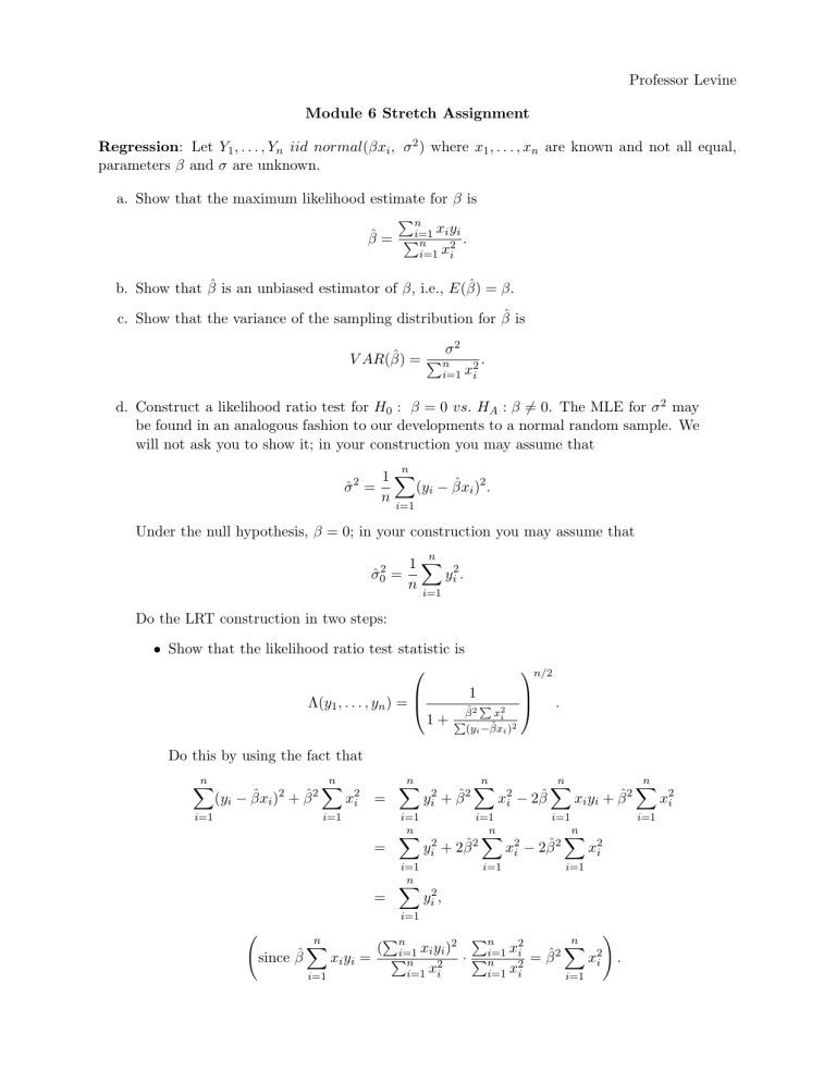
Professor Levine
Module 6 Stretch Assignment
Regression: Let Y1 , . . . , Yn iid normal(βxi , σ 2 ) where x1 , . . . , xn are known and not all equal,
parameters β and σ are unknown.
a. Show that the maximum likelihood estimate for β is
Pn
xi yi
β̂ = Pi=1
n
2 .
i=1 xi
b. Show that β̂ is an unbiased estimator of β, i.e., E(β̂) = β.
c. Show that the variance of the sampling distribution for β̂ is
σ2
V AR(β̂) = Pn
2.
i=1 xi
d. Construct a likelihood ratio test for H0 : β = 0 vs. HA : β 6= 0. The MLE for σ 2 may
be found in an analogous fashion to our developments to a normal random sample. We
will not ask you to show it; in your construction you may assume that
n
1X
σ̂ =
(yi − β̂xi )2 .
n
2
i=1
Under the null hypothesis, β = 0; in your construction you may assume that
n
σ̂02 =
1X 2
yi .
n
i=1
Do the LRT construction in two steps:
• Show that the likelihood ratio test statistic is


Λ(y1 , . . . , yn ) = 
n/2
1
1+
P 2
β̂ 2
xi
P
(yi −β̂xi )2


.
Do this by using the fact that
n
n
n
n
n
n
X
X
X
X
X
X
2
2
2
2
2
2
2
(yi − β̂xi ) + β̂
xi =
yi + β̂
xi − 2β̂
xi yi + β̂
x2i
i=1
i=1
i=1
=
n
X
yi2 + 2β̂
i=1
i=1
=
n
X
i=1
n
X
2
i=1
x2i − 2β̂ 2
n
X
i=1
x2i
i=1
yi2 ,
i=1
n
X
!
P
Pn
n
2
X
( ni=1 xi yi )2
x
2
i
since β̂
xi yi = Pn
· Pi=1
x2i .
n
2
2 = β̂
x
x
i=1
i=1
i
i
i=1
i=1
• Show that the LRT rejection region of Λ(y1 , . . . , yn ) < k is equivalent to rejecting
when
|β̂|
rP
> c.
2
(yP
i −β̂xi )
x2i
Hint: The development follows very closely to the LRT we constructed for a
t-test, see the slides for the t-test videos in Module 5. The reason is that we
are testing a normal mean, the difference here is that the mean is a linear
function of the xi s.
e. Using all the parts above, argue that we can test the hypotheses H0 : β = 0 vs. HA :
β 6= 0 through a t-test using the test statistic
β̂
rP
.
(yi −P
β̂xi )2
(n−1) x2i
As part of your discussion, present the rejection region for the test with the appropriate
critical value from the t distribution.
f. The inference developed in the parts above is for a regression model with no intercept:
yi = βxi + ei .
This model assumes data yi is linearly related to known xi with unknown slope coefficient. But this linear relationship is not perfect, there is some random error ei iid
normal(0, σ 2 ). In practice, we estimate β based on the pairs (yi , xi ), i = 1, . . . , n. We
then can make a prediction of y for a new value of x, let us denote this as prediction
ŷ0 predicted at value x0 . The model for this prediction is then
y0 = βx0 + e0 ; e0 ∼ N (0, σ 2 )
and the prediction is made by
ŷ0 = β̂x0 .
Do three things:
• Show that E(ŷ0 − y0 ) = 0. (Hint: here e0 is a random variable and x0 is a known
constant.)
• Show that
x0
V AR(ŷ0 − y0 ) = σ 2 1 + Pn
2
i=1 xi
.
• Argue that we can construct a confidence interval for y0 based on a critical value
from the t distribution. As part of your discussion, present the formula for a
(1 − α) confidence interval on y0 . Hint: The development follows analogously to
the construction of the t-interval for a normal mean. The difference here is that
our random variable is ŷ0 . Argue that ŷ0 is normally distributed and review the
slides for a confidence interval for the mean as part of the videos in Module 4.
g. The development in this problem is predicated on the normal model assumed for Yi with
linear mean βxi . If this model is not normal and further the relationship between yi and
xi is non-linear, discuss two ways we can develop a confidence interval on a parameter
β characterizing the relationship. Hint: Recall that we can approach inferences asymptotically or through simulation. You do not have to provide mathematical details, just
discuss how these two approaches can be used to construct confidence intervals, citing
relevant theorems/methods.
Note for the R Lab Practical: The development here is for a simple linear regression model with
no intercept and a single “independent variable” xi . In general, we will assume an intercept, so
yi ∼ normal(β0 + β1 xi , σ 2 ), i = 1, . . . , n. And further, we may have more than one independent
variable, say x1 , x2 , . . . , xp . The construction of inferences for the parameters and for prediction is
analogous, though with multiple parameters and multiple independent variables we must resort to
matrix algebra and calculus therein. For those of you who have taken a linear algebra course, you
can find the details in the Rice textbook Chapter 14. That said, for the R Lab Practical we will
fit a simple linear regression model with two parameters: an intercept term and a slope term. You
will not need to know the matrix theory to do that, and I will step you through the appropriate R
coding in the lab R Markdown file.