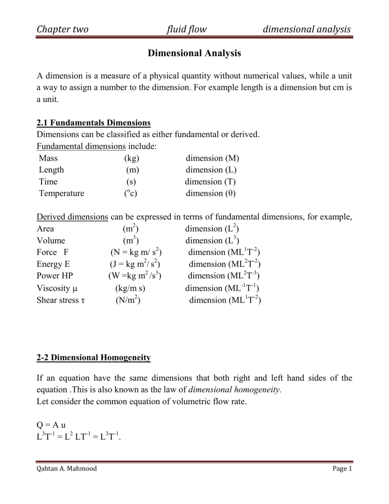
Chapter two
fluid flow
dimensional analysis
Dimensional Analysis
A dimension is a measure of a physical quantity without numerical values, while a unit
a way to assign a number to the dimension. For example length is a dimension but cm is
a unit.
2.1 Fundamentals Dimensions
Dimensions can be classified as either fundamental or derived.
Fundamental dimensions include:
Mass
(kg)
dimension (M)
Length
(m)
dimension (L)
Time
(s)
dimension (T)
o
Temperature
( c)
dimension (θ)
Derived dimensions can be expressed in terms of fundamental dimensions, for example,
Area
(m2)
dimension (L2)
Volume
(m3)
dimension (L3)
Force F
(N = kg m/ s2)
dimension (ML1T-2)
Energy E
(J = kg m2/ s2)
dimension (ML2T-2)
Power HP
(W =kg m2 /s3)
dimension (ML2T-3)
Viscosity 
(kg/m s)
dimension (ML-1T-1)
Shear stress τ
(N/m2)
dimension (ML1T-2)
2-2 Dimensional Homogeneity
If an equation have the same dimensions that both right and left hand sides of the
equation .This is also known as the law of dimensional homogeneity.
Let consider the common equation of volumetric flow rate.
Q=Au
L3T-1 = L2 LT-1 = L3T-1.
Qahtan A. Mahmood
Page 1
Chapter two
fluid flow
dimensional analysis
Example (2.1)
a) Determine the dimensions of the following quantities in M-L-T system 1- force 2pressure 3- work 4- power 5- surface tension 6- discharge 7- torque 8- momentum.
b) Check the dimensional homogeneity of the following equations
√
1-
2-
√

Solution:
a)
1- F = m.g
2- P=F/A
3- Work = F.distance
4- Power = Work/time
5-Surface tension = F/L
6-Discharge (Q)
7- Torque (Γ) = F.distance
8- Moment =
(kg.m/s2)
(N/m2) (Pa)
(N.m)
(W)
(N/m)
(m3/s)
(N.m)
(N.m )
≡ [MLT-2]
≡ [ML-1T-2]
≡ [ML2T-2]
≡ [ML-1T-2]
≡ [ML-1T-2]
≡ [L3T-1]
≡ [ML2T-2]
≡ [ML2T-2]
B)
1)
√
L.H.S. u ≡ [LT-1]
R.H.S. u ≡ *
+
= [LT-1]
Since the dimensions on both sides of the equation are same, therefore the equation is
dimensionally homogenous.
Qahtan A. Mahmood
Page 2
Chapter two
2)
fluid flow
dimensional analysis
√
L.H.S. Q ≡ [L3T-1]
R.H.S. (LT-2)1/2 (L)5/2 ≡ [L3T-1]
This equation is dimensionally homogenous.
Example (2-2)
If P is pressure and u is velocity and  is density what are the dimension in (MLT
system) for a) P/
b) pu
c) p/u2
Solution:
2-3 Methods of Dimensional Analysis
Many methods of dimensional analysis are available; two of these methods are given
here, which are:
1- Rayleigh’s method (or Power series)
2- Buckingham’s method (or Π-Theorem)
Qahtan A. Mahmood
Page 3
Chapter two
fluid flow
dimensional analysis
2.3.1 Rayleigh’s method (or Power series)
The Rayleigh’s method is based on the following steps:1- First of all, write the functional relationship with the given data.
2- Write the equation in terms of a constant with exponents i.e. powers a, b, c...
3- With the help of the principle of dimensional homogeneity, find out the values of a,
b, c … by obtaining simultaneous equation and simplify it.
4-Now substitute the values of these exponents in the main equation, and simplify it.
Example (2.3)
If the capillary rise (h) depends upon the specific weight (sp.wt) surface tension ( ) of
the liquid and tube radius (r) show that:
*
+ where φ is any function
Solution:
Capillary rise (h) m
Specific weight (sp.wt) N/m3 (MLT-2 L-3)
Surface tension (σ) N/m (MLT-2 L-1)
Tube radius (r) m
≡ [L]
≡ [ML-2T-2]
≡ [MT-2]
≡ [L]
h = f (sp.wt., σ, r)
h = k (sp.wt.a, σb, rc)
[L] = [ML-2T-2]a [MT-2]b[L]c
Now by the principle of dimensional homogeneity, equating the power of M, L, T on
both sides of the equation
For M
0=a+b
⇒ a=–b
For L
1=–2a+c
⇒ a=–b
For T
0=–2a–2b
⇒ a=–b
Qahtan A. Mahmood
Page 4
Chapter two
fluid flow
dimensional analysis
h = k (sp.wt.-b, σb, r1-2b)
[
]
Example (2.4)
Prove that the resistance (F) of a sphere of diameter (d) moving at a constant speed (u)
through a fluid density (ρ) and dynamic viscosity (μ) may be expressed as:
Solution:
Resistance (F) N
Diameter (d) m
Speed (u) m/s
Density (ρ) kg/m3
Viscosity (μ) kg/m.s
≡ [MLT-2]
≡ [L]
≡ [LT-1]
≡ [ML-3]
≡ [ML-1 T-1]
F = f (d, u, ρ, μ)
F = k (da, ub, ρc, μd)
[MLT-2] = [L]a [LT-1]b[ML-3]c[ML-1T-1]d
For M
For L
For T
1=c+d
1 = a + b – 3c – d
–2=–b–d
⇒ c =1 – d ----------------(1)
----------------(2)
⇒ b = 2 – d ----------------(3)
By substituting equations (1) and (3) in equation (2) give
a = 1 – b + 3c + d = 1 – (2 – d) + 3 (1 – d) + d = 2 – d
F = k (d2-d, u2-d, ρ1-d, μd)
= k (d2 u2 ρ) (μ / ρ u d)d
Example (2-5)
The pressure difference (AP) between two ends of a pipe in which a fluid is flowing is a
function of the pipe diameter d, the pipe length L, the fluid velocity u, the fluid density
p, and the fluid viscosity .
Solution:
Qahtan A. Mahmood
Page 5
Chapter two
fluid flow
dimensional analysis
p = f (L, d, ρ ,u, , μ)
p = k (La, db, ρc, ud, μe)
[ML-1 T-2] = [L]a [L]b[ML-3]c [LT-1]d[ML-1T-1]e
For M
For L
For T
1=c+e
⇒ c =1 – e
-1 = a + b – 3c + d– e
–2=–d–e
⇒d=2–e
--------(1)
--------(2)
--------(3)
By substituting equations (1) and (3) in equation (2) give
-1 = a + b – 3(1-e) + (2-e)-e
0= a +b+e
b= a + e
p = k (La, d-a-e, ρ1-e, u2-e μe)
2.3.2 Buckingham’s method (or Π-Theorem)
The Buckingham’s Π-theorem is based on the following steps:
Step 1. Identify the relevant variables
Step 2. Write down dimensions.
Step 3. Establish the number of independent dimensions and non-dimensional groups.
Number of relevant variables:
n=6
Number of independent dimensions:
m = 3 (M, L and T)
Number of non-dimensional groups (Πs):
n–m=3
Step 4. Choose m (= 3) dimensionally-independent scaling variables
Step 5. Create the Πs by non-dimensionalising the remaining variables
Qahtan A. Mahmood
Page 6
Chapter two
fluid flow
dimensional analysis
Guidelines for choosing repeating parameters in step 4 of the method of repeating
variables
 Never pick two parameters with the same dimensions or with dimensions that
differ by an exponent
 Never pick parameters that are already dimensionless.
 The chosen repeating must represent all the dimensions in the problem.
 The chosen repeating parameters must not by themselves be able to form a
dimensionless group to generate the rest of the Πs.
Example (2.6)
By dimensional analysis, obtain an expression for the drag force (F) on a partially
submerged body moving with a relative velocity (u) in a fluid; the other variables being
the linear dimension (L), surface roughness (), fluid density (ρ), and gravitationl
acceleration (g).
Solution:
F = k (u, L, , ρ, g)
f (F, u, L, , ρ, g) = 0
≡ [MLT-2]
≡ [LT-1]
≡ [L]
≡ [L]
≡ [ML-3]
≡ [L-1 T-2]
Drag force (F) N
Relative velocity (u) m/s
Linear dimension (L) m
Surface roughness () m
Density (ρ)
Acceleration of gravity (g) m
n = 6, m = 3,
⇒Π=n–m=6–3=3
No. of repeating variables = m = 3
The selected repeating variables is (u, L, ρ)
Π1 = ua1 Lb1 ρc1 F
Qahtan A. Mahmood
--------------(1)
Page 7
Chapter two
fluid flow
Π2 = ua2 Lb2 ρc2 
Π3 = ua3 Lb3 ρc3 g
dimensional analysis
--------------(2)
--------------(3)
For Π1 equation (1)
[M0 L0 T0] = [L T-1] a1 [L] b1 [ML-3] c1 [MLT-2]
Now applied dimensional homogeneity
For M
0 = c1 + 1
For T
0 = – a1 – 2
For L
0 = a1 + b1 – 3c1+ 1
-2 -2 -1
Π1 = u L ρ F
⇒ c1 = – 1
⇒ a1 = – 2
⇒ b1 = – 2
u
For Π2 equation (2)
[M0 L0 T0] = [L T-1] a2 [L] b2 [ML-3] c2 [L]
For M
For T
For L
0 = c2
0 = – a2
0 = a2 + b2 – 3c2+ 1
⇒ c2 = 0
⇒ a2 = 0
⇒ b2 = – 1
Π2 = L-1 

For Π3 equation (3)
[M0 L0 T0] = [L T-1]a3 [L]b3[ML-3]c3[L T-2]
For M
0 = c3
For T
0 = – a3 – 2
For L
0 = a3 + b3 – 3c3+ 1
-2
Π3 = u L g
⇒ c3 = 0
⇒ a3 = – 2
⇒ b3 = 1
g
u
f1 (Π 1, Π 2, Π 3) = 0
Qahtan A. Mahmood
Page 8
Chapter two
(

fluid flow
dimensional analysis
)

u
g
u
Example (2.7)
Prove that the discharge (Q) over a spillway ( ‫ )قناة لتصريف فائض المياه من سد او نهر‬is given
by the relation
u
√
u
Where: (u) velocity of flow (D) depth at the throat, (H), head of water, and (g)
gravitational acceleration.
Solution:
Q = k (u, D, H, g)
f (Q, u, D, H, g) = 0
Discharge (Q) m3/s
Velocity (u) m/s
Depth (D) m
Head of water (H) m
Acceleration of gravity (g) m/s2
n = 5, m = 2,
≡ [L3T-1]
≡ [LT-1]
≡ [L]
≡ [L]
≡ [ML-1 T-1]
⇒Π=n–m=5–2=3
No. of repeating variables = m = 2
The selected repeating variables is (u, D)
Π1 = ua1 Db1 Q
Π2 = ua2 Db2 H
Π3 = ua3 Db3 g
--------------(1)
--------------(2)
--------------(3)
For Π1 equation (1)
[M0 L0 T0] = [L T-1]a1 [L]b1[L3T-1]
Qahtan A. Mahmood
Page 9
Chapter two
For T
For L
Π1 = u-1 D-2 Q
fluid flow
dimensional analysis
⇒ a1 = – 1
⇒ b1 = – 2
0 = – a1 – 1
0 = a1 + b1 +3
u
For Π2 equation (2)
[M0 L0 T0] = [L T-1]a2 [L]b2[L]
For T
0 = – a2
For L
0 = a2 + b2 + 1
-1
Π2 = D H
⇒ a2 = 0
⇒ b2 = – 1
For Π3 equation (3)
[M0 L0 T0] = [L T-1]a3 [L]b3 [L T-2]
For T
0 = – a3 – 2
⇒ a3 = – 2
For L
0 = a3 + b3 + 1
⇒ b3 = 1
Π3 = u-2 D g
g
√
u
f1 (Π 1, Π 2, Π 3) = 0
f (
√
)
√
Example (2.8)
Show that the discharge of a centrifugal pump is given by
g
f
where (N) is the speed of the pump in r.p.m., (D) the diameter of impeller, (g)
gravitational acceleration, (H) manometric head, (μ), (ρ) are the dynamic viscosity and
the density of the fluid.
Solution:
Q = k (N, D, g, H, μ, ρ)
Qahtan A. Mahmood
Page 10
Chapter two
fluid flow
dimensional analysis
f (Q, N, D, g, H, μ, ρ) = 0
≡ [L3T-1]
≡ [T-1]
≡ [L]
≡ [ML-1 T-1]
≡ [L]
≡ [ML-1 T-1]
≡ [ML-3]
Discharge (Q) m3/s
Pump speed (N) r.p.m.
Diameter of impeller (D) m
Acceleration of gravity (g) m/s2
Head of manometer (H) m
Viscosity (μ) kg/m.s
Density (ρ) kg/m3
n = 7, m = 3,
⇒Π=n–m=7–3=4
No. of repeating variables = m = 3
The selected repeating variables is (N, D, ρ)
Π1 = Na1 Db1 ρc1 Q
Π2 = Na2 Db2 ρc2 g
Π3 = Na3 Db3 ρc3 H
Π4 = Na4 Db4 ρc4 μ
--------------(1)
--------------(2)
--------------(3)
--------------(4)
For Π1 equation (1)
[M0 L0 T0] = [T-1]a1 [L]b1[ML-3]c1[L3 T-1]
For M
0 = c1
⇒ c1 = 0
For T
0 = – a1 – 1
⇒ a1 = – 1
For L
0 = b1 – 3c1+ 3
⇒ b1 = – 3
Π1 = N-1 D-3 Q
For Π2 equation (2)
[M0 L0 T0] = [T-1]a2 [L]b2[ML-3]c2[LT-2]
For M
0 = c2
⇒ c2 = 0
For T
0 = – a2 – 2
⇒ a2 = – 2
Qahtan A. Mahmood
Page 11
Chapter two
For L
fluid flow
0 = b2 – 3c2+ 1
dimensional analysis
⇒ b2 = – 1
Π2 = N-2 D-1 g
g
For Π3 equation (3)
[M0 L0 T0] = [T-1]a3 [L]b3[ML-3]c3[L]
For M
0 = c3
⇒ c3 = 0
For T
0 = – a3
⇒ a3 = 0
For L
0 = b3 – 3c3+ 1
⇒ b3 = – 1
Π3 = D-1 H
For Π3 equation (4)
[M0 L0 T0] = [T-1]a4 [L]b4[ML-3]c4[ML-1T-1]
For M
0 = c4 + 1
⇒ c4 = – 1
For T
0 = – a4 – 1
⇒ a4 = – 1
For L
0 = b4 – 3c4 – 1
⇒ b4 = – 2
Π4 = N-1 D-2 ρ-1 μ
f1 (Π 1, Π 2, Π 3, Π 4) = 0
f (
)
(
Qahtan A. Mahmood
)
Page 12
Chapter two
fluid flow
dimensional analysis
2.5 Dimensions of some important variables
Item
Property
Symbol
SI Units
M.L.T.
1-
Velocity
u
m/s
LT-1
2-
Angular velocity
ω
Rad/s, Deg/s
T-1
3-
Rotational velocity
N
Rev/s
T-1
4-
Acceleration
a, g
m/s2
LT-2
5-
Angular acceleration
α
s-2
T-2
6-
Volumetric flow rate
Q
m3/s
L3T-1
7-
Discharge
Q
m3/s
L3T-1
8-
Mass flow rate
kg/s
MT-1
9-
Mass (flux) velocity
G
kg/m2.s
ML-2T-1
10-
Density
ρ
kg/m3
ML-3
11-
Specific volume
υ
m3/kg
L3M
12-
Specific weight
sp.wt
N/m3
ML-2T-2
13-
Specific gravity
sp.gr
[-]
[-]
14-
Dynamic viscosity
μ
kg/m.s, Pa.s
ML-1T-1
15-
Kinematic viscosity
ν
m2/s
L2T-1
16-
Force
F
N
MLT-2
17-
Pressure
P
N/m2≡Pa
ML-1T-2
18-
Pressure gradient
ΔP/L
Pa/m
ML-2T-2
19-
Shear stress
τ
N/m2
ML-1T-2
20-
Shear rate
γ
s-1
T-1
Qahtan A. Mahmood
m
Page 13
Chapter two
fluid flow
dimensional analysis
21-
Momentum
M
kg.m/s
MLT-1
22-
Work
W
N.m ≡J
ML2T-2
23-
Moment
M
N.m ≡J
ML2T-2
24-
Torque
Γ
N.m ≡J
ML2T-2
25-
Energy
E
J
ML2T-2
26-
Power
P
J/s ≡W
ML2T-3
27-
Surface tension
σ
N/m
MT-2
28-
Efficiency
η
[-]
[-]
29-
Head
h
m
L
30-
Modulus of elasticity
ε, K
Pa
ML-1T-2
Qahtan A. Mahmood
Page 14