Data Exploration, Visualization, and Feature
Engineering using R
Yuhui Zhang, and Raja Iqbal
Basic plotting systems
1. Base graphics: constructed piecemeal. Conceptually simpler and allows plotting to mirror the thought
process.
2. Lattice graphics: entire plots created in a simple function call.
3. ggplot2 graphics: an implementation of the Grammar of Graphics by Leland Wikinson. Combines
concepts from both base and lattice graphics. (Need to install ggplot2 library)
4. Fancier and more telling ones.
A list of interactive visualization in R can be found at:
interactive-visualizations.html
http://ouzor.github.io/blog/2014/11/21/
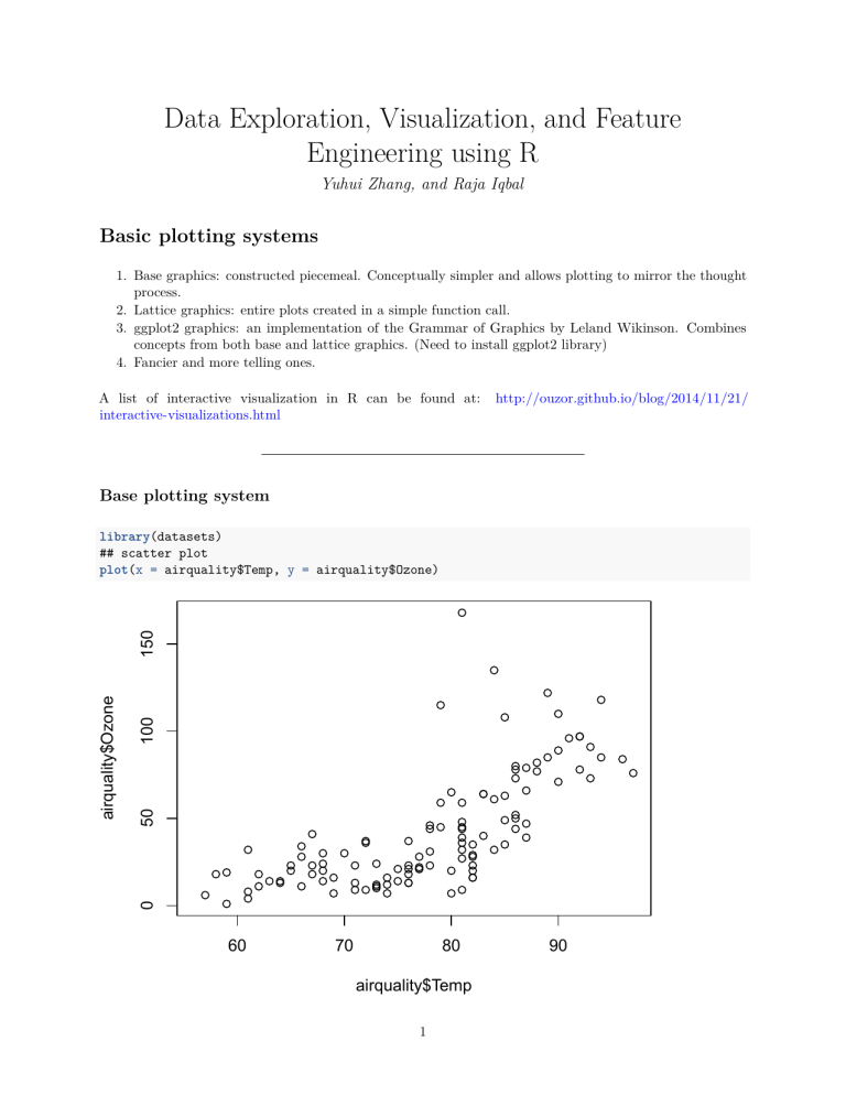
Base plotting system
100
50
0
airquality$Ozone
150
library(datasets)
## scatter plot
plot(x = airquality$Temp, y = airquality$Ozone)
60
70
80
airquality$Temp
1
90
Base plotting system
## par() function is used to specify global graphics parameters that affect all plots in an R session.
## Type ?par to see all parameters
par(mfrow = c(1, 2), mar = c(4, 4, 2, 1), oma = c(0, 0, 2, 0))
with(airquality, {
plot(Wind, Ozone, main="Ozone and Wind")
plot(Temp, Ozone, main="Ozone and Temperature")
mtext("Ozone and Weather in New York City", outer=TRUE)})
Ozone and Weather in New York City
100
0
50
Ozone
100
0
50
Ozone
150
Ozone and Temperature
150
Ozone and Wind
5
10
15
20
60
Wind
70
80
90
Temp
Plotting functions (high level)
PHASE ONE: Mount a canvas panel on the easel, and draw the draft. (Initialize a plot.)
• plot(): one of the most frequently used plotting functions in R.
• boxplot(): a boxplot show the distribution of a vector. It is very useful to example the distribution of
different variables.
• barplot(): create a bar plot with vertical or horizontal bars.
• hist(): compute a histogram of the given data values.
• pie(): draw a pie chart.
Remember to use ?plot or str(plot), etc. to check the arguments when you want to make more personalized
plots. A tutorial of base plotting system with more details: http://bcb.dfci.harvard.edu/~aedin/courses/
BiocDec2011/2.Plotting.pdf
Plotting functions (low level)
PHASE TWO: Add more details on your canvas, and make an artwork. (Add more on an existing
plot.)
• lines: adds liens to a plot, given a vector of x values and corresponding vector of y values
2
•
•
•
•
•
points: adds a point to the plot
text: add text labels to a plot using specified x,y coordinates
title: add annotations to x,y axis labels, title, subtitles, outer margin
mtext: add arbitrary text to margins (inner or outer) of plot
axis: specify axis ticks
Save your artwork
R can generate graphics (of varying levels of quality) on almost any type of display or printing device. Like:
• postscript(): for printing on PostScript printers, or creating PostScript graphics files.
• pdf(): produces a PDF file, which can also be included into PDF files.
• jpeg(): produces a bitmap JPEG file, best used for image plots.
help(Devices) for a list of them all. Simple example:
## png(filename = 'plot1.png', width = 480, height = 480, units = 'px')
## plot(x, y)
## dev.off()
Example: boxplot and hitogram
## the layout
par(mfrow = c(2, 1), mar = c(2, 0, 2, 0), oma = c(0, 0, 0, 0))
## histogram at the top
hist(airquality$Ozone, breaks=12, main = "Histogram of Ozone")
## box plot below for comparison
boxplot(airquality$Ozone, horizontal=TRUE, main = "Box plot of Ozone")
3
Histogram of Ozone
0
50
100
150
Box
plot of Ozone
airquality$Ozone
0
50
100
150
Lattice plotting system
library(lattice) # need to load the lattice library
set.seed(10) # set the seed so our plots are the same
x <- rnorm(100)
f <- rep(1:4, each = 25) # first 25 elements are 1, second 25 elements are 2, ...
y <- x + f - f * x+ rnorm(100, sd = 0.5)
f <- factor(f, labels = c("Group 1", "Group 2", "Group 3", "Group 4"))
# first 25 elements are in Group 1, second 25 elements are in Group 2, ...
xyplot(y ~ x | f)
−2
Group 1
−1
0
1
2
−2
Group 2
Group 3
6
y
4
2
0
−2
−1
0
1
2
−2
x
Lattice plotting system
Want more on the plot? Customize the panel funciton:
4
−1
0
0
Group 4
8
−2
−1
1
2
1
2
xyplot(y ~ x | f, panel = function(x, y, ...) {
# call the default panel function for xyplot
panel.xyplot(x, y, ...)
# adds a horizontal line at the median
panel.abline(h = median(y), lty = 2)
# overlays a simple linear regression line
panel.lmline(x, y, col = 2)
})
Lattice plotting system
−2
Group 3
−1
0
1
2
Group 4
8
6
4
2
0
−2
y
Group 1
Group 2
8
6
4
2
0
−2
−2
−1
0
1
2
x
Lattice plotting system
Plotting functions * xyplot(): main function for creating scatterplots * bwplot(): box and whiskers plots
(box plots) * histogram(): histograms * stripplot(): box plot with actual points * dotplot(): plot dots on
“violin strings” * splom(): scatterplot matrix (like pairs() in base plotting system) * levelplot()/contourplot():
plotting image data
5
Very useful when we want a lot. . .
pairs(iris) ## iris is a data set in R
3.0
4.0
0.5
1.5
2.5
6.5
2.0
3.5
4.5
Sepal.Length
5
7
2.0
Sepal.Width
2.0
1
3
Petal.Length
1.0 2.0 3.0
0.5
Petal.Width
Species
4.5
6.0
7.5
1
3
5
7
1.0
2.0
3.0
ggplot2
• An implementation of the Grammar of Graphics by Leland Wikinson
• Written by Hadley Wickham (while he was a graduate student as lowa State)
• A “third” graphics system for R (along with base and lattice)
Available from CRAN via install.packages()
web site: http://ggplot2.org (better documentation)
• Grammar of graphics represents the abstraction of graphics ideas/objects
Think “verb”, “noun”, “adjective” for graphics
“Shorten” the distance from mind to page
• Two main functions:
qplot() hides what goes on underneath, which is okay for most operations ggplot() is the core function
and very flexible for doing this qplot() cannot do
qplot function
The qplot() function is the analog to plot() but with many build-in features
Syntax somewhere in between base/lattice
Difficult to be customized (don’t bother, use full ggplot2 power in that case)
6
library(ggplot2) ## need to install and load this library
qplot(displ, hwy, data = mpg, facets = .~drv)
4
f
r
hwy
40
30
20
2
3
4
5
6
7
2
3
4
5
6
7
2
3
4
5
6
displ
ggplot function
When building plots in ggplot2 (ggplot, rather than using qplot)
The “artist’s palette” model may be the closest analogy
Plots are built up in layers
Step I: Input the data
noun: the data
library(ggplot2) ## need to install and load this library
g <- ggplot(iris, aes(Sepal.Length, Sepal.Width)) ## this would not show you add plot
ggplot function
• Step II: Add layers
adjective: describe the type of plot you will produce.
g + geom_point() + geom_smooth(method = "lm") + facet_grid(. ~ Species)
7
7
setosa
4.5
versicolor
virginica
Sepal.Width
4.0
3.5
3.0
2.5
2.0
5
6
7
8
5
6
7
8
5
6
7
8
7
8
Sepal.Length
ggplot function
• Step III: Add metadata and annotation
adjective: control the mapping between data and aesthetics.
g <- g + geom_point() + geom_smooth(method = "lm") + facet_grid(. ~ Species)
g + ggtitle("Sepal length vs. width for different species") + theme_bw() ## verb
Sepal length vs. width for different species
setosa
4.5
versicolor
virginica
Sepal.Width
4.0
3.5
3.0
2.5
2.0
5
6
7
8
5
6
7
8
5
Sepal.Length
Great documentation
Great documentation of ggplot with all functions in step II and III and demos:
http://docs.ggplot2.org/current/
8
6
Titanic tragedy data
Reading RAW training data
• Download the data set “Titanic_train.csv” from https://raw.githubusercontent.com/datasciencedojo/
datasets/master/Titanic_train.csv
• Set working directory of R to the directory of the file using setwd()
titanic = read.csv('Titanic_train.csv')
Look at the first few rows
What would be some good features to consider here?
options(width = 110)
head(titanic)
##
##
##
##
##
##
##
##
##
##
##
##
##
##
1
2
3
4
5
6
1
2
3
4
5
6
PassengerId Survived Pclass
Name
Sex Age SibSp Pa
1
0
3
Braund, Mr. Owen Harris
male 22
1
2
1
1 Cumings, Mrs. John Bradley (Florence Briggs Thayer) female 38
1
3
1
3
Heikkinen, Miss. Laina female 26
0
4
1
1
Futrelle, Mrs. Jacques Heath (Lily May Peel) female 35
1
5
0
3
Allen, Mr. William Henry
male 35
0
6
0
3
Moran, Mr. James
male NA
0
Ticket
Fare Cabin Embarked
A/5 21171 7.2500
S
PC 17599 71.2833
C85
C
STON/O2. 3101282 7.9250
S
113803 53.1000 C123
S
373450 8.0500
S
330877 8.4583
Q
What is the data type of each column?
sapply(titanic,class)
## PassengerId
##
"integer"
##
Fare
##
"numeric"
Survived
"integer"
Cabin
"factor"
Pclass
"integer"
Embarked
"factor"
Name
"factor"
9
Sex
"factor"
Age
"numeric"
SibSp
"integer"
Parch
"integer"
"f
Converting class label to a factor
titanic$Survived = factor(titanic$Survived, labels=c("died", "survived"))
titanic$Embarked = factor(titanic$Embarked, labels=c("unkown", "Cherbourg", "Queenstown", "Southampton")
sapply(titanic,class)
## PassengerId
##
"integer"
##
Fare
##
"numeric"
Survived
"factor"
Cabin
"factor"
Pclass
"integer"
Embarked
"factor"
Name
"factor"
Sex
"factor"
str(titanic$Survived)
##
Factor w/ 2 levels "died","survived": 1 2 2 2 1 1 1 1 2 2 ...
str(titanic$Sex)
##
Factor w/ 2 levels "female","male": 2 1 1 1 2 2 2 2 1 1 ...
Class distribution - PIE Charts
survivedTable = table(titanic$Survived)
survivedTable
##
##
##
died survived
549
342
par(mar = c(0, 0, 0, 0), oma = c(0, 0, 0, 0))
pie(survivedTable,labels=c("Died","Survived"))
Died
Survived
10
Age
"numeric"
SibSp
"integer"
Parch
"integer"
"f
Is Sex a good predictor?
male = titanic[titanic$Sex=="male",]
female = titanic[titanic$Sex=="female",]
par(mfrow = c(1, 2), mar = c(0, 0, 2, 0), oma = c(0, 1, 0, 1))
pie(table(male$Survived),labels=c("Dead","Survived"), main="Survival Portion Among Men")
pie(table(female$Survived),labels=c("Dead","Survived"), main="Survival Portion Among Women")
Survival Portion Among Men
Survival Portion Among Women
Dead
Dead
Survived
Survived
Is Age a good predictor?
Age <- titanic$Age; summary(Age)
##
##
Min. 1st Qu.
0.42
20.12
Median
28.00
Mean 3rd Qu.
29.70
38.00
Max.
80.00
How about summary segmented by survival
summary(titanic[titanic$Survived=="0",]$Age)
##
##
Min. 1st Qu.
Median
Mean 3rd Qu.
Max.
summary(titanic[titanic$Survived=="1",]$Age)
##
##
Min. 1st Qu.
Median
Mean 3rd Qu.
Max.
Age distribution by Survival and Sex
11
NA's
177
par(mfrow = c(1, 2), mar = c(4, 4, 2, 2), oma = c(1, 1, 1, 1))
boxplot(titanic$Age~titanic$Sex, main="Age Distribution By Gender",col=c("red","green"))
boxplot(titanic$Age~titanic$Survived, main="Age Distribution By Survival",col=c("red","green"),
xlab="0:Died 1:Survived",ylab="Age")
60
40
20
0
0
20
40
Age
60
80
Age Distribution By Survival
80
Age Distribution By Gender
female
male
died
survived
0:Died 1:Survived
Histogram of Age
hist(Age, col="blue", xlab="Age", ylab="Frequency",
main = "Distribution of Passenger Ages on Titanic")
12
100
0
50
Frequency
150
200
Distribution of Passenger Ages on Titanic
0
20
40
60
80
Age
Kernel density plot of age
d = density(na.omit(Age)) # density(Age) won't work, need to omit all NAs
plot(d, main = "kernel density of Ages of Titanic Passengers")
polygon(d, col="red", border="blue")
13
0.020
0.000
0.010
Density
0.030
kernel density of Ages of Titanic Passengers
0
20
40
60
80
N = 714 Bandwidth = 3.226
Comparison of density plots of Age with different Sex
## Package 'sm', version 2.2-5.4: type help(sm) for summary information
14
Kernel Density Plot of Ages By Sex
0.000
0.010
Density
0.020
0.030
female
male
−20
0
20
40
60
80
100
Age of Passenger
Did Age have an impact on survival?
Kernel Density Plot of Ages By Survival
0.035
Kernel Density Plot of Ages By Sex
0.035
kernel density of Ages of Titanic Passengers
died
survived
0.025
Density
0.020
0.020
Density
0
20
40
60
80
0.010
0.000
0.000
0.000
0.005
0.005
0.005
0.010
0.015
0.015
0.015
0.010
Density
0.020
0.025
0.025
0.030
0.030
0.030
female
male
−20
N = 714 Bandwidth = 3.226
0
20
40
60
Age of Passenger
Create categorical groupings: Adult vs Child
An example of feature engineering!
## Multi dimensional comparison
Child <- titanic$Age # Isolating age.
15
80
100
−20
0
20
40
Age of Passenger
60
80
100
## Now we need to create categories: NA = Unknown, 1 = Child, 2 = Adult
## Every age below 13 (exclusive) is classified into age group 1
Child[Child<13] <- 1
## Every child 13 or above is classified into age group 2
Child[Child>=13] <- 2
# Use labels instead of 0's and 1's
Child[Child==1] <- "Child"
Child[Child==2] <- "Adult"
# Appends the new column to the titanic dataset
titanic_with_child_column <- cbind(titanic, Child)
# Removes rows where age is NA
titanic_with_child_column <- titanic_with_child_column[!is.na(titanic_with_child_column$Child),]
Fare matters?
Adult
Child
500
400
female
300
200
Fare
100
0
500
400
male
300
200
100
0
died
survived
died
Survived
***
16
survived
How about fare, ship class, port embarkation?
unkown
Cherbourg
Queenstown
Southampton
500
400
Fare
300
200
100
0
1
2
3
1
2
3
1
2
3
Pclass
Diamond data
Overview of the diamond data
data(diamonds) # loading diamonds data set
head(diamonds, 16) # first few rows of diamond data set
##
##
##
##
##
##
##
##
##
##
##
##
##
##
##
##
##
1
2
3
4
5
6
7
8
9
10
11
12
13
14
15
16
carat
0.23
0.21
0.23
0.29
0.31
0.24
0.24
0.26
0.22
0.23
0.30
0.23
0.22
0.31
0.20
0.32
cut color clarity depth table price
x
y
z
Ideal
E
SI2 61.5
55
326 3.95 3.98 2.43
Premium
E
SI1 59.8
61
326 3.89 3.84 2.31
Good
E
VS1 56.9
65
327 4.05 4.07 2.31
Premium
I
VS2 62.4
58
334 4.20 4.23 2.63
Good
J
SI2 63.3
58
335 4.34 4.35 2.75
Very Good
J
VVS2 62.8
57
336 3.94 3.96 2.48
Very Good
I
VVS1 62.3
57
336 3.95 3.98 2.47
Very Good
H
SI1 61.9
55
337 4.07 4.11 2.53
Fair
E
VS2 65.1
61
337 3.87 3.78 2.49
Very Good
H
VS1 59.4
61
338 4.00 4.05 2.39
Good
J
SI1 64.0
55
339 4.25 4.28 2.73
Ideal
J
VS1 62.8
56
340 3.93 3.90 2.46
Premium
F
SI1 60.4
61
342 3.88 3.84 2.33
Ideal
J
SI2 62.2
54
344 4.35 4.37 2.71
Premium
E
SI2 60.2
62
345 3.79 3.75 2.27
Premium
E
I1 60.9
58
345 4.38 4.42 2.68
Histogram of carat
17
1
2
3
library(ggplot2)
ggplot(data=diamonds) + geom_histogram(aes(x=carat))
## stat_bin: binwidth defaulted to range/30. Use 'binwidth = x' to adjust this.
count
7500
5000
2500
0
0
2
4
carat
Density plot of carat
ggplot(data=diamonds) +
geom_density(aes(x=carat),fill="gray50")
18
density
1.5
1.0
0.5
0.0
0
1
2
3
carat
Scatter plots (carat vs. price)
ggplot(diamonds, aes(x=carat,y=price)) + geom_point()
19
4
5
price
15000
10000
5000
0
0
1
2
3
4
carat
Carat with colors
g = ggplot(diamonds, aes(x=carat, y=price)) # saving first layer as variable
g + geom_point(aes(color=color)) # rendering first layer and adding another layer
20
5
15000
color
D
price
E
F
10000
G
H
I
J
5000
0
0
1
2
3
carat
Carat with colors (more details)
g + geom_point(aes(color=color)) + facet_wrap(~color)
21
4
5
D
E
F
G
H
I
15000
10000
5000
0
color
D
price
15000
E
F
10000
G
H
5000
I
J
0
J
15000
10000
5000
0
0
1
2
3
4
5
carat
Let’s consider cut and clarity
I1
SI2
SI1
VS2
VS1
VVS2
VVS1
IF
15000
Fair
10000
5000
0
15000
Good
10000
5000
color
0
D
price
Very Good
15000
10000
5000
E
F
G
H
I
0
J
15000
Premium
10000
5000
0
15000
Ideal
10000
5000
0
0
1
2
3
4
5 0
1
2
3
4
5 0
1
2
3
4
5 0
1
2
3
4
5 0
carat
22
1
2
3
4
5 0
1
2
3
4
5 0
1
2
3
4
5 0
1
2
3
4
5
Your trun!
What is your knowledge of diamond’s price after exploring this data?
Interactive visualization in R - rCharts
• What is rCharts?
Is an R package to create, customize and publish interactive javascript visualizations from R using a
familiar lattice style plotting interface.
• What rCharts can make and how?
Quick start at: http://ramnathv.github.io/rCharts/
• A list of interactive visualization in R can be found at:
http://ouzor.github.io/blog/2014/11/21/interactive-visualizations.html
Tell your story - R Markdown
• R Markdown is an authoring format that enables easy creation of dynamic documents, presentations,
and reports from R.
• It combines the core syntax of markdown (an easy-to-write plain text format) with embedded R code
chunks that are run so their output can be included in the final document.
• Many available output formats including HTML, PDF, and MS Word
• Installation
Use RStudio: already installed
Outside of RStudio: install.packages(“rmarkdown”). A recent version of pandoc (>= 1.12.3) is also
required. See https://github.com/rstudio/rmarkdown/blob/master/PANDOC.MD to install it.
Check out Markdown first
Markdown is a markup language with plain text formatting syntax designed so that it can be
converted to HTML and many other formats using a tool by the same name.
One minute you get the point, and always check the cheat sheets
https://github.com/adam-p/markdown-here/wiki/Markdown-Cheatsheet#lists
23
Then, R Markdown sample code
Download the template:
https://github.com/datasciencedojo/datasets/blob/master/rmarkdownd_template.Rmd
R Markdown
• YAML header
• Edit Markdown, and R chunks
• Run!
RStudio: knitr button
Command line: render(“file.Rmd”)
Cheat sheet of rmarkdown:
http://www.rstudio.com/wp-content/uploads/2015/02/rmarkdown-cheatsheet.pdf
Present your story of Titanic!
Use * Titanic data * Plotting functions in R * R Markdown template * The heart of data explorer
to write your story of Titanic. . .
Hope this is inspiring :)
Titanic
24