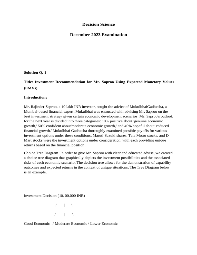
Decision Science
December 2023 Examination
Solution Q. 1
Title: Investment Recommendation for Mr. Saproo Using Expected Monetary Values
(EMVs)
Introduction:
Mr. Rajinder Saproo, a 10 lakh INR investor, sought the advice of MukulbhaiGadhecha, a
Mumbai-based financial expert. Mukulbhai was entrusted with advising Mr. Saproo on the
best investment strategy given certain economic development scenarios. Mr. Saproo's outlook
for the next year is divided into three categories: 10% positive about 'genuine economic
growth,' 50% confident about'moderate economic growth,' and 40% hopeful about 'reduced
financial growth.' Mukulbhai Gadhecha thoroughly examined possible payoffs for various
investment options under these conditions. Maruti Suzuki shares, Tata Motor stocks, and D
Mart stocks were the investment options under consideration, with each providing unique
returns based on the financial position.
Choice Tree Diagram: In order to give Mr. Saproo with clear and educated advise, we created
a choice tree diagram that graphically depicts the investment possibilities and the associated
risks of each economic scenario. The decision tree allows for the demonstration of capability
outcomes and expected returns in the context of unique situations. The Tree Diagram below
is an example.
Investment Decision (10, 00,000 INR)
/
|
\
/
|
\
Good Economic / Moderate Economic \ Lower Economic
Growth
/
Growth
\
Growth
10% (0.10) /
50% (0.50)
\
/
\
/
/
\
/
40% (0.40)
/
\
/
/
\
/
Mauti Suzuki Shares TATA Motor Shares D Mart shares
3, 00,000 (0.10)
4, 00,000 (0.10)
|
|
1, 20,000 (0.50)
|
50,000 (0.40)
|
1,00,000 (0.50)
|
4,50,000 (0.10)
2,30,000 (0.50)
|
10,000 (0.40)
30,000 (0.40)
The decision tree displays Mr. Saproo's choices, which are entirely based on his available
money of 10,000 INR and the probability assigned to each economic development scenario.
The three investment possibilities are set out on the tree's last degree, each with its own return
for 'genuine financial increase,''moderate financial growth,' and 'decreased financial rise.'
EMVs (Expected Monetary Values):
We estimated the anticipated economic Values (EMVs) for each financing choice for each
economic scenario to arrive at a good funding decision for Mr. Saproo. EMV is an important
decision-making tool since it takes into account both capacity returns and their related
possibilities. EMV is computed as the product and probability of each conceivable end
outcome.
Here are the EMVs calculated for each investment option:
Mauti Suzuki Shares:
EMV = (0.10 * 3, 00,000) + (0.50 * 1, 20,000) + (0.40 * 50,000) = 30,000 + 60,000 + 20,000
= 110,000 INR
TATA Motor shares:
EMV = (0.10 * 4, 00,000) + (0.50 * 1, 00,000) + (0.40 * 10,000) = 40,000 + 50,000 + 4,000
= 94,000 INR
D Mart shares:
EMV = (0.10 * 4, 50,000) + (0.50 * 2,30,000) + (0.40 * 30,000) = 45,000 + 1,15,000 +
12,000 = 172,000 INR
Recommendations:
D-Mart stock is Mr. Saproo's favorite investment, as is his EMV calculation for most of all
investment options. This feature gives you the highest estimated return on most investments,
with an EMV of approximately INR 172,000. Of partners
D Mart aims to maximize efficiency while evaluating relevant opportunities. The
recommendations are based on a comprehensive analysis of recovery plans under different
financial development scenarios identified in the EMV.
result:
To summarize, Mr. Tapulo proposed to invest Rs 1 million and select D-Mart shares. Support
this desire by carefully considering the possibilities and potential returns of each financial
option. By specializing in D-Mart stock, Mr. Saplow is able to maximize profits depending
on his optimistic view of the financial future, as shown by the probabilities he assigns to
different economic growth scenarios. However, Sapro said it is important to keep in mind
that all investments involve a certain level of risk, and that market conditions should be
disclosed in order to make informed decisions as circumstances change. You should continue
to do so and regularly review your investment portfolio. This recommendation is primarily
based on the information available at the time of the decision and an understanding of the
economic scenario.
SOLUTION - 2
The Quest for the Optimal Alpha:
Within the field of forecasting, we set out on a journey to discover the alpha value, which
holds the secret to greater predictive abilities. Our path leads us through the thick forest of
mean Absolute Deviation (MAD) and the perilous terrain of suggest-squared errors (MSE).
These measurements will be our compass on our journey.
The Participants:
Our worthy adversaries are alpha values 0.1, 0.2, 0.5, 0.7, and 0.9. Each Alpha strives to
establish its value in the realm of predicting, but only one will triumph.
Alpha = 0.1
(1)
(2)
(3)
r
s
(α=0.1)
2
1127 0.1⋅977+0.9⋅977=977
3
694
4
1357 0.1⋅694+0.9⋅992=962.2
5
1020 0.1⋅1357+0.9⋅962.2=1001.68
6
1187 0.1⋅1020+0.9⋅1001.68=1003.512
7
866
yea Sale Exponential Smoothing
1
8
977
1459
977
0.1⋅1127+0.9⋅977=992
0.1⋅1187+0.9⋅1003.512=1021.8608
0.1⋅866+0.9⋅1021.8608=1006.2747
9
1163 0.1⋅1459+0.9⋅1006.2747=1051.5472
10
991
11
1411 0.1⋅991+0.9⋅1062.6925=1055.5233
12
1323 0.1⋅1411+0.9⋅1055.5233=1091.0709
13
995
14
1764 0.1⋅995+0.9⋅1114.2638=1102.3375
15
1552 0.1⋅1764+0.9⋅1102.3375=1168.5037
16
1465 0.1⋅1552+0.9⋅1168.5037=1206.8533
17
1398 0.1⋅1465+0.9⋅1206.8533=1232.668
18
1893 0.1⋅1398+0.9⋅1232.668=1249.2012
19
1422 0.1⋅1893+0.9⋅1249.2012=1313.5811
20
2063 0.1⋅1422+0.9⋅1313.5811=1324.423
21
1703 0.1⋅2063+0.9⋅1324.423=1398.2807
22
1758 0.1⋅1703+0.9⋅1398.2807=1428.7526
23
0.1⋅1758+0.9⋅1428.7526=1461.6774
(1) (2)
yea Sal
r
1
2
es
0.1⋅1163+0.9⋅1051.5472=1062.6925
0.1⋅1323+0.9⋅1091.0709=1114.2638
(3)
Exponential
Smoothing
(4)
Error
(5)
|Error|
(6)
Error2
977 977
112
7
977
1127-977=150
150
22500
(7)
|%Erro
r|
13.31%
3
4
5
6
7
8
9
10
11
12
13
14
15
16
17
694 992
135
7
102
0
118
7
694-992=-298
298
88804
42.94%
962.2
1357-962.2=394.8
394.8
155867.04
29.09%
1001.68
1020-1001.68=18.32
18.32
335.6224
1.8%
1003.512
866 1021.8608
145
9
116
3
1006.2747
1051.5472
991 1062.6925
141
1
132
3
1055.5233
1091.0709
995 1114.2638
176
4
155
2
146
5
1102.3375
1168.5037
1206.8533
139 1232.668
1187-
1003.512=183.488
183.488 33667.8461 15.46%
866-1021.8608=-
155.860
1459-
452.725 204960.179
155.8608
1006.2747=452.7253
1163-
1051.5472=111.4528
991-1062.6925=71.6925
8
3
111.452
8
24292.589
2
71.6925 5139.8179
355.476 126363.704
1323-
231.929
1091.0709=231.9291
995-1114.2638=119.2638
1764-
1102.3375=661.6625
1552-
1168.5037=383.4963
1465-
1206.8533=258.1467
1398-
7
1
119.263
8
9
25.19%
14223.8658 11.99%
5
9
3
3
383.496 147069.398
7
7.23%
53791.0871 17.53%
661.662 437797.310
258.146
31.03%
12421.7159 9.58%
1411-
1055.5233=355.4767
18%
37.51%
24.71%
66639.6949 17.62%
165.332 27334.6664 11.83%
8
18
19
20
21
22
189
3
142
2
206
3
170
3
175
8
23
1232.668=165.332
1249.2012
1313.5811
1324.423
1398.2807
1428.7526
1461.6774
1893-
643.798 414476.881
1422-
108.418
1249.2012=643.7988
1313.5811=108.4189
2063-
1324.423=738.577
8
9
738.577
4
11754.6602 7.62%
545496.013
8
1703-
304.719
1758-
329.247 108403.841
1398.2807=304.7193
1428.7526=329.2474
Total
Forecasting errors
3
(1)
(2)
(3)
r
s
(α=0.2)
2
1127 0.2⋅977+0.8⋅977=977
yea Sale Exponential Smoothing
1
977
977
35.8%
92853.8625 17.89%
4
1
79
78
18.73%
6136.40 2594193.79 428.88
1. Mean absolute error (MAE), also called mean absolute deviation (MAD)
2. Mean squared error (MSE)
34.01%
%
0.2⋅1127+0.8⋅977=1007
3
694
4
1357 0.2⋅694+0.8⋅1007=944.4
5
1020 0.2⋅1357+0.8⋅944.4=1026.92
6
1187 0.2⋅1020+0.8⋅1026.92=1025.536
7
866
8
1459 0.2⋅866+0.8⋅1057.8288=1019.463
9
1163 0.2⋅1459+0.8⋅1019.463=1107.3704
10
991
11
1411 0.2⋅991+0.8⋅1118.4963=1092.9971
12
1323 0.2⋅1411+0.8⋅1092.9971=1156.5977
13
995
14
1764 0.2⋅995+0.8⋅1189.8781=1150.9025
15
1552 0.2⋅1764+0.8⋅1150.9025=1273.522
16
1465 0.2⋅1552+0.8⋅1273.522=1329.2176
17
1398 0.2⋅1465+0.8⋅1329.2176=1356.3741
18
1893 0.2⋅1398+0.8⋅1356.3741=1364.6993
19
1422 0.2⋅1893+0.8⋅1364.6993=1470.3594
20
2063 0.2⋅1422+0.8⋅1470.3594=1460.6875
21
1703 0.2⋅2063+0.8⋅1460.6875=1581.15
22
1758 0.2⋅1703+0.8⋅1581.15=1605.52
23
0.2⋅1187+0.8⋅1025.536=1057.8288
0.2⋅1163+0.8⋅1107.3704=1118.4963
0.2⋅1323+0.8⋅1156.5977=1189.8781
0.2⋅1758+0.8⋅1605.52=1636.016
(1) (2)
yea Sal
r
1
2
3
4
5
6
7
8
9
10
11
12
13
es
(3)
Exponential
Smoothing
(4)
Error
(5)
|Error|
(6)
Error2
977 977
112
7
977
7
102
0
118
7
9
116
3
22500
13.31%
694-1007=-313
313
97969
45.1%
944.4
1357-944.4=412.6
412.6
170238.76
30.41%
1026.92
1020-1026.92=-6.92
6.92
47.8864
0.68%
1025.536
1019.463
1107.3704
991 1118.4963
141
1
132
3
r|
150
866 1057.8288
145
|%Erro
1127-977=150
694 1007
135
(7)
1092.9971
1156.5977
995 1189.8781
1187-
1025.536=161.464
866-1057.8288=191.8288
1459-
1019.463=439.537
1163-
1107.3704=55.6296
161.464 26070.6233 13.6%
191.828
8
439.537
36798.2885 22.15%
193192.739
2
55.6296 3094.6488
991-1118.4963=-
127.496
1411-
318.002 101125.859
127.4963
1092.9971=318.0029
1323-
1156.5977=166.4023
995-1189.8781=194.8781
3
9
166.402
3
194.878
1
30.13%
4.78%
16255.3181 12.87%
4
22.54%
27689.7384 12.58%
37977.4851 19.59%
14
15
16
17
18
19
20
21
22
23
176
4
155
2
146
5
139
8
189
3
142
2
206
3
170
3
175
8
1150.9025
1273.522
1329.2176
1356.3741
1364.6993
1470.3594
1764-
1150.9025=613.0975
1552-
1273.522=278.478
1465-
1329.2176=135.7824
1398-
1356.3741=41.6259
1893-
1364.6993=528.3007
1422-1470.3594=48.3594
613.097 375888.540
5
6
34.76%
278.478 77549.9951 17.94%
135.782
4
18436.8596 9.27%
41.6259 1732.7171
528.300 279101.666
7
3
48.3594 2338.6328
2.98%
27.91%
3.4%
2063-
602.312 362780.311
5
8
1581.15
1703-1581.15=121.85
121.85
14847.4167 7.16%
1605.52
1758-1605.52=152.48
152.48
23250.1446 8.67%
1636.016
Total
1460.6875
1460.6875=602.3125
5060.04 1888886.63
54
17
Forecasting errors
1. Mean absolute error (MAE), also called mean absolute deviation (MAD)
2. Mean squared error (MSE)
29.2%
369%
Alpha = 0.5
(1)
(2)
(3)
r
s
(α=0.5)
2
1127 0.5⋅977+0.5⋅977=977
3
694
4
1357 0.5⋅694+0.5⋅1052=873
5
1020 0.5⋅1357+0.5⋅873=1115
6
1187 0.5⋅1020+0.5⋅1115=1067.5
7
866
8
1459 0.5⋅866+0.5⋅1127.25=996.625
9
1163 0.5⋅1459+0.5⋅996.625=1227.8125
10
991
11
1411 0.5⋅991+0.5⋅1195.4062=1093.2031
12
1323 0.5⋅1411+0.5⋅1093.2031=1252.1016
13
995
14
1764 0.5⋅995+0.5⋅1287.5508=1141.2754
15
1552 0.5⋅1764+0.5⋅1141.2754=1452.6377
16
1465 0.5⋅1552+0.5⋅1452.6377=1502.3188
17
1398 0.5⋅1465+0.5⋅1502.3188=1483.6594
18
1893 0.5⋅1398+0.5⋅1483.6594=1440.8297
yea Sale Exponential Smoothing
1
977
977
0.5⋅1127+0.5⋅977=1052
0.5⋅1187+0.5⋅1067.5=1127.25
0.5⋅1163+0.5⋅1227.8125=1195.4062
0.5⋅1323+0.5⋅1252.1016=1287.5508
19
1422 0.5⋅1893+0.5⋅1440.8297=1666.9149
20
2063 0.5⋅1422+0.5⋅1666.9149=1544.4574
21
1703 0.5⋅2063+0.5⋅1544.4574=1803.7287
22
1758 0.5⋅1703+0.5⋅1803.7287=1753.3644
23
0.5⋅1758+0.5⋅1753.3644=1755.6822
(1) (2)
yea Sal
r
1
2
3
4
5
6
7
8
9
10
es
(3)
Exponential
Smoothing
(4)
Error
(5)
|Error|
(6)
Error2
977 977
112
7
977
7
102
0
118
7
9
116
3
r|
150
22500
13.31%
694-1052=-358
358
128164
51.59%
873
1357-873=484
484
234256
35.67%
1115
1020-1115=-95
95
9025
9.31%
1067.5
1187-1067.5=119.5
119.5
14280.25
10.07%
866-1127.25=-261.25
261.25
68251.5625 30.17%
866 1127.25
145
|%Erro
1127-977=150
694 1052
135
(7)
996.625
1227.8125
991 1195.4062
1459-996.625=462.375 462.375
1163-1227.8125=64.8125
991-1195.4062=-
213790.640
6
64.8125 4200.6602
204.406
41781.915
31.69%
5.57%
20.63%
11
12
13
14
15
16
17
18
19
20
21
22
23
141
1
132
3
1093.2031
1252.1016
995 1287.5508
176
4
155
2
146
5
139
8
189
3
142
2
206
3
170
3
175
8
1141.2754
1452.6377
1502.3188
1483.6594
1440.8297
1666.9149
1544.4574
1803.7287
1753.3644
1755.6822
204.4062
2
1093.2031=317.7969
9
14111323-
1252.1016=70.8984
317.796 100994.853
8
70.8984 5026.5884
995-1287.5508=-
292.550
1764-
622.724 387785.939
292.5508
1141.2754=622.7246
1552-
1452.6377=99.3623
1465-1502.3188=37.3188
1398-1483.6594=85.6594
8
6
1
6.4%
37.3188 1392.6964
2.55%
85.6594 7337.5369
6.13%
1422-1666.9149=-
244.914
2063-
1544.4574=518.5426
1703-1803.7287=100.7287
1758-
1753.3644=4.6356
Total
35.3%
99.3623 9872.8676
452.170 204457.969
244.9149
5.36%
85585.9596 29.4%
1893-
1440.8297=452.1703
22.52%
3
9
518.542
6
100.728
7
4.6356
4
23.89%
59983.2867 17.22%
268886.399 25.14%
10146.2738 5.91%
21.4892
0.26%
5046.64 1877741.88 388.09
71
82
%
Forecasting errors
1. Mean absolute error (MAE), also called mean absolute deviation (MAD)
MAD =5046.6471 / 21=240.3165
2. Mean squared error (MSE)
MSE=1877741.8882 / 21=89416.2804
ALPHA = 0.7
(1)
(2)
(3)
r
s
(α=0.7)
2
1127 0.7⋅977+0.3⋅977=977
3
694
4
1357 0.7⋅694+0.3⋅1082=810.4
5
1020 0.7⋅1357+0.3⋅810.4=1193.02
6
1187 0.7⋅1020+0.3⋅1193.02=1071.906
7
866
8
1459 0.7⋅866+0.3⋅1152.4718=951.9415
9
1163 0.7⋅1459+0.3⋅951.9415=1306.8825
10
991
11
1411 0.7⋅991+0.3⋅1206.1647=1055.5494
yea Sale Exponential Smoothing
1
977
977
0.7⋅1127+0.3⋅977=1082
0.7⋅1187+0.3⋅1071.906=1152.4718
0.7⋅1163+0.3⋅1306.8825=1206.1647
12
1323 0.7⋅1411+0.3⋅1055.5494=1304.3648
13
995
14
1764 0.7⋅995+0.3⋅1317.4094=1091.7228
15
1552 0.7⋅1764+0.3⋅1091.7228=1562.3169
16
1465 0.7⋅1552+0.3⋅1562.3169=1555.0951
17
1398 0.7⋅1465+0.3⋅1555.0951=1492.0285
18
1893 0.7⋅1398+0.3⋅1492.0285=1426.2086
19
1422 0.7⋅1893+0.3⋅1426.2086=1752.9626
20
2063 0.7⋅1422+0.3⋅1752.9626=1521.2888
21
1703 0.7⋅2063+0.3⋅1521.2888=1900.4866
22
1758 0.7⋅1703+0.3⋅1900.4866=1762.246
23
0.7⋅1758+0.3⋅1762.246=1759.2738
(1) (2)
yea Sal
r
1
2
3
4
5
es
0.7⋅1323+0.3⋅1304.3648=1317.4094
(3)
Exponential
Smoothing
(4)
Error
(5)
|Error|
(6)
Error2
977 977
112
7
977
7
102
0
|%Erro
r|
1127-977=150
150
22500
13.31%
694-1082=-388
388
150544
55.91%
810.4
1357-810.4=546.6
546.6
298771.56
40.28%
1193.02
1020-1193.02=-173.02
173.02
29935.9204 16.96%
694 1082
135
(7)
6
7
8
9
10
11
12
13
14
15
16
17
18
19
118
7
1071.906
866 1152.4718
145
9
116
3
951.9415
1306.8825
991 1206.1647
141
1
132
3
1055.5494
1304.3648
995 1317.4094
176
4
155
2
146
5
139
8
189
3
142
2
1091.7228
1562.3169
1555.0951
1492.0285
1426.2086
1752.9626
1187-
1071.906=115.094
115.094 13246.6288 9.7%
866-1152.4718=-
286.471
1459-
507.058 257108.281
286.4718
951.9415=507.0585
1163-1306.8825=143.8825
991-1206.1647=215.1647
1411-
1055.5494=355.4506
1323-
1304.3648=18.6352
8
5
143.882
5
215.164
7
82066.0922 33.08%
9
20702.1629 12.37%
46295.8647 21.71%
355.450 126345.113
6
7
18.6352 347.2697
995-1317.4094=-
322.409 103947.852
1764-
672.277 451956.587
322.4094
1091.7228=672.2772
1552-1562.3169=10.3169
1465-1555.0951=90.0951
1398-1492.0285=94.0285
4
1
2
4
1.41%
32.4%
38.11%
0.66%
90.0951 8117.119
6.15%
94.0285 8841.3619
6.73%
466.791 217894.253
1422-1752.9626=-
330.962 109536.220
330.9626
25.19%
10.3169 106.4374
1893-
1426.2086=466.7914
34.75%
4
2
6
4
24.66%
23.27%
20
21
22
206
3
170
3
175
8
23
1521.2888
1900.4866
2063-
541.711 293451.056
1703-1900.4866=-
197.486
1521.2888=541.7112
197.4866
1762.246
1758-1762.246=-4.246
1759.2738
Total
2
6
4.246
8
39000.9694 11.6%
18.0284
21
03
1. Mean absolute error (MAE), also called mean absolute deviation (MAD)
2. Mean squared error (MSE)
MSE=2280732.7803 / 21=108606.3229
ALPHA = 0.9
(1)
(2)
(3)
r
s
(α=0.9)
2
1127 0.9⋅977+0.1⋅977=977
3
694
4
1357 0.9⋅694+0.1⋅1112=735.8
5
1020 0.9⋅1357+0.1⋅735.8=1294.88
6
1187 0.9⋅1020+0.1⋅1294.88=1047.488
yea Sale Exponential Smoothing
1
977
977
0.9⋅1127+0.1⋅977=1112
0.24%
5629.70 2280732.78 434.76
Forecasting errors
MAD=5629.7021 / 21=268.0811
26.26%
%
0.9⋅1187+0.1⋅1047.488=1173.0488
7
866
8
1459 0.9⋅866+0.1⋅1173.0488=896.7049
9
1163 0.9⋅1459+0.1⋅896.7049=1402.7705
10
991
11
1411 0.9⋅991+0.1⋅1186.977=1010.5977
12
1323 0.9⋅1411+0.1⋅1010.5977=1370.9598
13
995
14
1764 0.9⋅995+0.1⋅1327.796=1028.2796
15
1552 0.9⋅1764+0.1⋅1028.2796=1690.428
16
1465 0.9⋅1552+0.1⋅1690.428=1565.8428
17
1398 0.9⋅1465+0.1⋅1565.8428=1475.0843
18
1893 0.9⋅1398+0.1⋅1475.0843=1405.7084
19
1422 0.9⋅1893+0.1⋅1405.7084=1844.2708
20
2063 0.9⋅1422+0.1⋅1844.2708=1464.2271
21
1703 0.9⋅2063+0.1⋅1464.2271=2003.1227
22
1758 0.9⋅1703+0.1⋅2003.1227=1733.0123
23
0.9⋅1758+0.1⋅1733.0123=1755.5012
(1) (2)
yea Sal
r
1
es
0.9⋅1163+0.1⋅1402.7705=1186.977
0.9⋅1323+0.1⋅1370.9598=1327.796
(3)
Exponential
Smoothing
977 977
(4)
Error
(5)
|Error|
(6)
Error2
(7)
|%Erro
r|
2
3
4
5
6
7
8
9
10
11
12
13
14
15
16
112
7
977
1127-977=150
150
22500
13.31%
694-1112=-418
418
174724
60.23%
735.8
1357-735.8=621.2
621.2
385889.44
45.78%
1294.88
1020-1294.88=-274.88
274.88
75559.0144 26.95%
694 1112
135
7
102
0
118
7
1047.488
866 1173.0488
145
9
116
3
896.7049
1402.7705
991 1186.977
141
1
132
3
1010.5977
1370.9598
995 1327.796
176
4
155
2
1028.2796
1690.428
146 1565.8428
1187-
1047.488=139.512
139.512 19463.5981 11.75%
866-1173.0488=-
307.048
1459-
562.295
307.0488
896.7049=562.2951
1163-1402.7705=239.7705
991-1186.977=195.977
1411-
1010.5977=400.4023
1323-1370.9598=47.9598
995-1327.796=332.796
1764-
1028.2796=735.7204
1552-1690.428=138.428
1465-1565.8428=-
8
1
239.770
5
94278.9656 35.46%
316175.802 38.54%
57489.8869 20.62%
195.977 38407.0037 19.78%
400.402 160321.997
3
9
47.9598 2300.1396
332.796
110753.162
3
735.720 541284.510
4
4
138.428 19162.3
28.38%
3.63%
33.45%
41.71%
8.92%
100.842 10169.2695 6.88%
5
17
18
19
20
21
22
23
139
8
189
3
142
2
206
3
170
3
175
8
100.8428
1475.0843
1405.7084
1844.2708
1464.2271
2003.1227
1733.0123
1755.5012
1398-1475.0843=77.0843
8
77.0843 5941.9862
1893-
487.291 237453.076
1422-1844.2708=-
422.270 178312.664
1405.7084=487.2916
422.2708
2063-
1464.2271=598.7729
1703-2003.1227=300.1227
1758-
1733.0123=24.9877
Total
6
2
8
7
9
6
598.772 358529.004
300.122
7
5.51%
25.74%
29.7%
29.02%
90073.6401 17.62%
24.9877 624.3866
1.42%
6575.36 2899413.84 504.39
27
88
%
Errors in forecasting
1. Mean absolute error (MAE), also known as mean absolute deviation (MAD), is defined as
MAD=6575.3627/21=313.1125
MSE (mean squared error)
MSE=2899413.8488/21=138067.3261
Let's now make a chart in MS Excel to show the MAD and MSE values for each alpha. Based
on these criteria, we will next examine which alpha is substantially better for the projection.
When we study the results, two alpha values jump out as strong contenders: 0.2 and 0.5. They
have the lowest MAD and MSE values, indicating their predicting accuracy. These alphas
have shown to be dependable friends in our pursuit of accuracy.
The Final Thought:
Alpha values of 0.2 and 0.5 have emerged as winners in the big forecasting arena, where
precision is important. Their ability to limit mistakes, both absolute and squared, makes them
the preferred choice for those seeking the most dependable forecasts.
In the long term, the choice of alpha is obvious: Allow 0.2 and 0.5 to lead the way in our
forecasting efforts, as they have shown to be the keys to unlocking.
SOLUTION 3-A
We dug into world data and regular distribution to determine the odds of the Mirchi set from
the product surviving 100 days. With a mean lifespan (mean) of 90 days and a standard
deviation of 10 days, we start calculating the difference using Z-scores for the fascinating
world of the ancient traditional line distribution table.
Step 1: Find the Z-score< br>Z-score is the knight in shining armor number, it is our guide to
help us understand how close the value is to the average. In this study, we investigated the Z
score of the 100-day durability of the Mirchi lamp. The Z-score is expressed by the following
expression:
Z = (X-μ) / σ
where:
X is the interest amount, 100 days.
µ, noble environment (life expectancy), stable at 90 days.
σ is the confidence level of the standard deviation, the 10-day confidence level
After calling this model, the Z score emerges:
Z=(100 -90)/ 2= 1< br>
2. Step: Uncovering the Possibility
With Z-scores, we plan to reveal hidden opportunities in the history of the common table.
These words correspond to ancient writings about Z-scores that reveal the secrets of
probability.
Our task is to show the probability that the Z score is not less than 1 but also equal to or less
than 1 ( P ( Z≤1 ) ). Normal distribution process, our estimate is uncertain and the famous P
(Z ≤ 1) is about 0.8413.
So the result is correct: there is an attractive probability of 0.8413 or 84.13%. Here's the
chance for the Mirchi sets selected from the batch to bravely last 100 days.
In conclusion, a journey into the mysterious world of statistics reveals a chance of 84.13%. It
is estimated that the Mirchi lighting selection from the manufacturer can withstand 100 days
of reviews and clicks, which is taken from the average and deals with different aspects of life
and is considered a normal distribution.
SOLUTION 3-B
Stacked Bar
14000
12000
10000
8000
6000
4000
2000
0
ALMORA
BAGESHWAR
CHAMOLI
CHAMPAWAT
DEHRADUN
HARIDWAR
Micro
NAINITAL
Small
PAURI GARHWAL
PITHORAGARH
RUDRA PRAYAG
TEHRI GARHWAL
UDHAM SINGH NAGAR
UTTARKASHI
Medium
Reasons for Choosing Stacked Bar Chart:
Comparative Clarity: The main objective is to have a clear and visible assessment of the
contribution of micro, small and medium enterprises to all MSMEs in every district of
Uttarakhand. Stacked bar charts do a good job of showing the contributions within each
section. This similarity is important to understand the distribution of MSME groups across
states.
Part-to-whole visualization: Stacked bar charts essentially show part-to-whole relationships.
Each bar in the chart represents all small, medium and micro businesses in a region. The
segments in this row represent 3 MSME categories: micro, small and medium. The
department facilitates all types of assistance to all MSMEs in a district. It's good to take
things apart.
Smart Information About the Region: Uttarakhand is a state where many economic changes
are taking place in its various regions. Stacked bar charts help compare the composition of
MSMEs across regions. By analyzing the share of micro, small and medium businesses in
each segment, stakeholders will benefit from understanding the type of business in the near
future. Based on this assessment, policy makers and experts can develop strategies for
different regions. Clarity and Accessibility: Stacked bar charts are known for their clarity and
ease of interpretation. They are intuitive and require little explanation. Each area is
represented by a bar, and sections of the bar are often shaded to increase clarity. This design
ensures that the image is usable and understandable by a variety of business targets,
regardless of whether they are familiar with data visualization techniques. Visual
differentiation through color coding significantly improves readability, allowing viewers to
easily differentiate between MSME groups.
Conclusion:
Stacked bar chart has been chosen as the required visualization method to show the
contribution of small and medium enterprises in Uttarakhand to small and medium
enterprises at several important points as follows: applicable. It provides a clear basis for
comparison, ensures a good communication of the space as a whole, compares between
regions, makes it understandable and accessible. This decision ensures that the truth is
presented in the lesson and understood by a wide audience; this makes it an excellent tool to
demonstrate understanding of the fragmentation of the MSME group in the state.