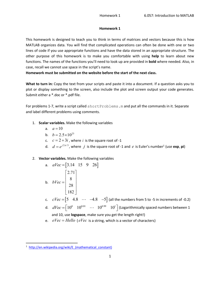
Homework 1
6.057: Introduction to MATLAB
Homework 1
This homework is designed to teach you to think in terms of matrices and vectors because this is how
MATLAB organizes data. You will find that complicated operations can often be done with one or two
lines of code if you use appropriate functions and have the data stored in an appropriate structure. The
other purpose of this homework is to make you comfortable with using help to learn about new
functions. The names of the functions you’ll need to look up are provided in bold where needed. Also, in
case, recall we cannot use space in the script’s name.
Homework must be submitted on the website before the start of the next class.
What to turn in: Copy the text from your scripts and paste it into a document. If a question asks you to
plot or display something to the screen, also include the plot and screen output your code generates.
Submit either a *.doc or *.pdf file.
For problems 1-7, write a script called shortProblems.m and put all the commands in it. Separate
and label different problems using comments.
1. Scalar variables. Make the following variables
a. a = 10
b. b = 2.5´1023
c. c = 2 + 3i , where i is the square root of -1
d.
d = e j 2p / 3 , where j is the square root of -1 and e is Euler’s number1 (use exp, pi)
2. Vector variables. Make the following variables
a.
aVec = [3.14 15 9 26]
é 2.71ù
ê 8 ú
ú
b. bVec = ê
ê 28 ú
ê
ú
ë 182 û
c. cVec = [5 4.8 ! -4.8 -5] (all the numbers from 5 to -5 in increments of -0.2)
d.
dVec = éë100 100.01 ! 100.99 101 ûù (Logarithmically spaced numbers between 1
and 10, use logspace, make sure you get the length right!)
e. eVec = Hello ( eVec is a string, which is a vector of characters)
1
http://en.wikipedia.org/wiki/E_(mathematical_constant)
1
Homework 1
6.057: Introduction to MATLAB
3. Matrix variables. Make the following variables
é2 !
ê
a. aMat = " #
ê
êë 2 !
é1 0
ê
ê0 "
b. bMat = ê # 0
ê
ê "
êë0
[1 2 3 4 5
c.
2ù
" úú a 9x9 matrix full of 2’s (use ones or zeros)
2 úû
!
0ù
0 " úú
5 0 # ú a 9x9 matrix of all zeros, but with the values
ú
0 " 0ú
! 0 1 úû
4 3 2 1] on the main diagonal (use zeros, diag).
é 1 11 ! 91 ù
ê 2 12 " 92 ú
ú a 10x10 matrix where the vector 1:100 runs down the
cMat = ê
ê#
# " # ú
ê
ú
ë10 20 ! 100 û
columns (use reshape).
é NaN NaN NaN
ê
d. dMat = NaN NaN NaN
ê
êë NaN NaN NaN
é 13 -1 5 ù
e. eMat = ê
ú
ë -22 10 -87 û
f.
NaN ù
NaN úú a 3x4 NaN matrix (use nan)
NaN úû
Make fMat be a 5x3 matrix of random integers with values on the range -3 to 3 (First
use rand and floor or ceil. Now only use randi)
4. Scalar equations. Using the variables created in 1, calculate x , y , and
a.
x=
b.
y=
z.
1
1+ e
(
( -( a -15) /6)
)
p
a + 21 b , recall that
g
h = h1/ g , and use sqrt. You can also use nthroot (refer
to the MATLAB help to understand the difference between nthroot and a fractional
power)
c.
(
)
log  éë( c + d )( c - d ) ùû sin ( ap / 3)
where  indicates the real part of the
cc
complex number in brackets, c is the complex conjugate of c , and log is the natural
z=
log (use real, conj, log).
2
Homework 1
6.057: Introduction to MATLAB
5. Matrix equations. Using the variables created in 2 and 3, find the values of xMat, yMat and
zMat below. Use matrix operators.
a. xMat = (aVec ∙ bVec) ∙ aMat b. yMat = (bVec ∙ aVec), note that this is not the same as (aVec ∙ bVec)
c. zMat = |cMat|(aMat ∙ bMat)1 , where cMat is the determinant of cMat , and T again
indicates the transpose (use det).
6. Common functions and indexing.
a. Make cSum the column-wise sum of cMat . The answer should be a row vector (use
sum).
b. Make eMean the mean across the rows of eMat . The answer should be a column (use
mean).
c. Replace the top row of eMat with [1 1 1] .
d. Make cSub the submatrix of cMat that only contains rows 2 through 9 and columns 2
through 9.
e. Make the vector lin = [1 2 ! 20] (the integers from 1 to 20), and then make
every even value in it negative to get lin = [1 -2 3 -4 ! -20] .
f.
Make r a 1x5 vector using rand. Find the elements that have values <0.5 and set those
values to 0 (use find).
7. Plotting multiple lines and colors. In class we saw how to plot a single line in the default blue
color on a plot. You may have noticed that subsequent plot commands simply replace the
existing line. Here, we’ll write a script to plot two lines on the same axes.
a. Open a script and name it twoLinePlot.m. Write the following commands in this
script.
b. Make a new figure using figure
c. We’ll plot a sine wave and a cosine wave over one period
i. Make a time vector t from 0 to 2p with enough samples to get smooth lines
ii. Plot sin ( t )
iii. Type hold on to turn on the ‘hold’ property of the figure. This tells the figure not
to discard lines that are already plotted when plotting new ones. Similarly, you
can use hold off to turn off the hold property.
iv. Plot cos ( t ) using a red dashed line. To specify line color and style, simply add a
third argument to your plot command (see the third paragraph of the plot help).
3
Homework 1
6.057: Introduction to MATLAB
This argument is a string specifying the line properties as described in the help
file. For example, the string ‘k:’ specifies a black dotted line.
d. Now, we’ll add labels to the plot
i. Label the x axis using xlabel
ii. Label the y axis using ylabel
iii. Give the figure a title using title
iv. Create a legend to describe the two lines you have plotted by using legend and
passing to it the two strings ‘Sin’ and ‘Cos’.
e. If you run the script now, you’ll see that the x axis goes from 0 to 7 and y goes from -1 to
1. To make this look nicer, we’ll manually specify the x and y limits. Use xlim to set the x
axis to be from 0 to 2p and use ylim to set the y axis to be from -1.4 to 1.4.
f. Run the script to verify that everything runs right. You should see something like this:
Sin and Cos functions
Sin
Cos
1
Function value
0.5
0
-0.5
-1
0
1
2
3
Time (s)
4
4
5
6
Homework 1
8.
6.057: Introduction to MATLAB
Manipulating variables. Write a script to read in some grades, curve them, and display the
overall grade. To do this, you’ll need to download the file classGrades.mat off the class
website and put it in the same folder as your script.
a. Open a script and name it calculateGrades.m. Write all the following commands
in this script.
b. Load the classGrades file using load. This file contains a single variable called
namesAndGrades
c. To see how namesAndGrades is structured, display the first 5 rows on your screen.
The first column contains the students ‘names’, they’re just the integers from 1 to 15.
The remaining 7 columns contain each student’s score (on a scale from 0 to 5) on each
of 7 assignments. There are also some NaNs which indicate that a particular student was
absent on that day and didn’t do the assignment.
d. We only care about the grades, so extract the submatrix containing all the rows but only
columns 2 through 8 and name this matrix grades (to make this work on any size
matrix, don’t hard-code the 8, but rather use end or size(namesAndGrades,2)).
e. Calculate the mean score on each assignment. The result should be a 1x7 vector
containing the mean grade on each assignment.
i. First, do this using mean. Display the mean grades calculated this way. Notice
that the NaNs that were in the grades matrix cause some of the mean grades to
be NaN as well.
ii. To fix this problem, do this again using nanmean. This function does exactly
what you want it to do, it computes the mean using only the numbers that are
not NaN. This means that the absent students are not considered in the
calculation, which is what we want. Name this mean vector meanGrades and
display it on the screen to verify that it has no NaNs
f. Normalize each assignment so that the mean grade is 3.5 (this is a B- on our 5 point
scale). You’ll want to divide each column of grades by the correct element of
meanGrades .
i. Make a matrix called meanMatrix such that it is the same size as grades , and
each row has the values meanGrades . Do this by taking the outer product of a
15x1 vector of ones and the vector meanGrades , which is a row (use ones, *).
Display meanMatrix to verify that it looks the way you want.
ii. To
calculate
the
curved
grades,
do
the
following:
curvedGrades = 3.5 ( grades / meanMatrix ) . Keep in mind that you want to
do the division elementwise.
iii. Compute and display the mean of curvedGrades to verify that they’re all 3.5
(nanmean).
iv. Because we divided by the mean and multiplied by 3.5, it’s possible that some
grades that were initially close to 5 are now larger than 5. To fix this, find all the
5
Homework 1
6.057: Introduction to MATLAB
elements in curvedGrades that are greater than 5 and set them to 5. Use
logical indexing and DO NOT use find.
g. Calculate the total grade for each student and assign letter grades
i. To calculate the totalGrade vector, which will contain the numerical grade for
each student, you want to take the mean of curvedGrades across the columns
(use nanmean, see help for how to specify the dimension). Also, we only want
to end up with numbers from 1 to 5, so calculate the ceiling of the totalGrade
vector (use ceil).
ii. Make a string called letters that contains the letter grades in increasing order:
FDCBA
iii. Make the final letter grades vector letterGrades by using totalGrade (which
after the ceil operation should only contain values between 1 and 5) to index
into letters .
iv. Finally, display the following using disp: Grades: letterGrades
h. Run the script to verify that it works. You should get an output like this
6
Homework 1
6.057: Introduction to MATLAB
Optional Problems
1. Throwing a ball. Below are all the steps you need to follow, but you should also add your own
meaningful comments to the code as you write it.
a. Start a new file in the MATLAB Editor and save it as throwBall.m
b. At the top of the file, define some constants (you can pick your own variable names)
i. Initial height of ball at release = 1.5 m
ii. Gravitational acceleration = 9.8 m/s2
iii. Velocity of ball at release = 4 m/s
iv. Angle of the velocity vector at time of release = 45 degrees
c. Next, make a time vector that has 1000 linearly spaced values between 0 and 1,
inclusive.
d. If x is distance and y is height, the equations below describe their dependence on
time and all the other parameters (initial height h , gravitational acceleration g , initial
ball velocity v , angle of velocity vector in degrees q ). Solve for x and y
p
æ p ö
to convert degrees to radians.
x ( t ) = v cos ç q
÷ t . We multiply q by
180
è 180 ø
æ p ö 1 2
ii. y ( t ) = h + v sin ç q
÷ t - gt
è 180 ø 2
i.
e. Approximate when the ball hits the ground.
i. Find the index when the height first becomes negative (use find).
ii. The distance at which the ball hits the ground is value of x at that index
iii. Display the words: The ball hits the ground at a distance of X meters. (where X is
the distance you found in part ii above)
f. Plot the ball’s trajectory
i. Open a new figure (use figure)
ii. Plot the ball’s height on the y axis and the distance on the x axis (plot)
iii. Label the axes meaningfully and give the figure a title (use xlabel, ylabel, and
title)
iv. Hold on to the figure (use hold on)
v. Plot the ground as a dashed black line. This should be a horizontal line going
from 0 to the maximum value of x (use max). The height of this line should be
0. (see help plot for line colors and styles)
g. Run the script from the command window and verify that the ball indeed hits the
ground around the distance you estimated in e-ii. You should get something like this:
7
Homework 1
6.057: Introduction to MATLAB
Ball Trajectory
2
1.5
Ball Height (m)
1
0.5
0
-0.5
-1
0
0.5
1
1.5
Distance (m)
8
2
2.5
3
Homework 1
6.057: Introduction to MATLAB
2. Convergence of infinite series. We’ll look at two series that converge to a finite value when they
are summed.
a. Open a new script in the MATLAB Editor and save it as seriesConvergence.m
b. First, we’ll deal with a geometric series G =
¥
åp
k
. We need to define the value of p
k =0
and the values of k
i. p =0.99.
ii. k is a vector containing the integers from 0 to 1000, inclusive.
c. Calculate each term in the series (before summation)
i.
geomSeries = p k (this should be done elementwise)
d. Calculate the value of the infinite series
i. We know that G =
¥
åp
k =0
k
=
1
1- p
e. Plot the value of the infinite series
i. Plot a horizontal red line that has x values 0 and the maximum value in k (use
max), and the y value is constant at G .
f. On the same plot, plot the value of the finite series for all values of k
i. Plot the cumulative sum of geomSeries versus k . The cumulative sum of a
vector is a vector of the same size, where the value of each element is equal to
the sum of all the elements to the left of it in the original vector. (use cumsum,
and try cumsum([1 1 1 1 1]) to understand what it’s doing.) Use a blue line when
plotting.
g. Label the x and y axes, and give the figure a title (xlabel, ylabel, title). Also create a
legend and label the first line ‘Infinite sum’, and the second line ‘Finite Sum’ (legend).
h. Run the script and note that the finite sum of 1000 elements comes very close to the
value of the infinite sum.
i.
Next, we will do a similar thing for another series, the p-series: P =
¥
1
ån
n=1
j.
p
At the bottom of the same script, initialize new variables
i. p = 2
ii. n is a vector containing all the integers from 1 to 500, inclusive.
k. Calculate the value of each term in the series
i.
l.
pSeries =
1
np
Calculate the value of the infinite p-series. The infinite p-series with p = 2 has been
proven to converge to P =
1 p2
= .
å
p
6
n=1 n
¥
9
Homework 1
6.057: Introduction to MATLAB
m. Make a new figure and plot the infinite sum as well as the finite sum, as we did for the
geometric series
i. Make a new figure
ii. Plot the infinite series value as a horizontal red line with x values 0 and the
maximum value in n , and the y value is constant at P .
iii. Hold on to the figure, and plot the cumulative sum of pSeries versus n (use
hold on, cumsum).
iv. Label the x and y axes, give the figure a title, and make a legend to label the
lines as ‘Infinite sum’, and ‘Finite sum’ (use xlabel, ylabel, title, legend)
n. Run the script to verify that it produces the expected output. It should look something
like this:
Convergence of geometric series with p=0.99
100
Infinite sum
Finite sum
90
80
70
Sum
60
50
40
30
20
10
0
0
100
200
300
400
500
Index
600
700
800
900
1000
Convergence of p-series with p=2
1.8
Infinite sum
Finite sum
1.7
1.6
Sum
1.5
1.4
1.3
1.2
1.1
1
0
50
100
150
200
250
Index
300
350
10
400
450
500
Homework 1
6.057: Introduction to MATLAB
3. Encryption Algorithm. Write a simple shuffling ‘encryption’ algorithm.
a. Open a new script and save it as encrypt.m
b. At the top of the script, define the original string to be: This is my top secret message!
c. Next, let’s shuffle the indices of the letters. To do this, we need to make a string of
encoding indices
i. Make a vector that has the indices from 1 to the length of the original string in a
randomly permuted order. Use randperm and length
ii. Encode the original string by using your encoding vector as indices into
original . Name the encoded message encoded .
d. Now, we need to figure out the decoding key to match the encoding key we just made.
i. Assemble a temporary matrix where the first column is the encoding vector you
made in the previous part and the second column are the integers from 1 to the
length of the original string in order. Use length, and you may need to transpose
some vectors to make them columns using ‘.
ii. Next, we want to sort the rows of this temporary matrix according to the values
in the first column. Use sortrows.
iii. After it’s been sorted, extract the second column of the temporary matrix. This
is your decoding vector.
iv. To make the decoded message, use the decoding vector as indices into
encoded .
e. Display the original, encoded, and decoded messages
i. Display the following three strings, where : original , encoded , and decoded
are the strings you made above. Use disp
Original: original
f.
Encoded: encoded
Decoded: decoded
Compare the original and decoded strings to make sure they’re identical and display the
result
i. Use strcmp to compare the original and decoded strings. Name the output
of this operation correct . correct will have the value 1 if the strings match
and the value 0 if they don’t
ii. Display the following string: Decoded correctly (1 true, 0 false): correct
use disp and num2str
g. Run the script a few times to verify that it works well. You should see an output like this:
11
MIT OpenCourseWare
https://ocw.mit.edu
6.057 Introduction to MATLAB
IAP 2019
For information about citing these materials or our Terms of Use, visit: https://ocw.mit.edu/terms