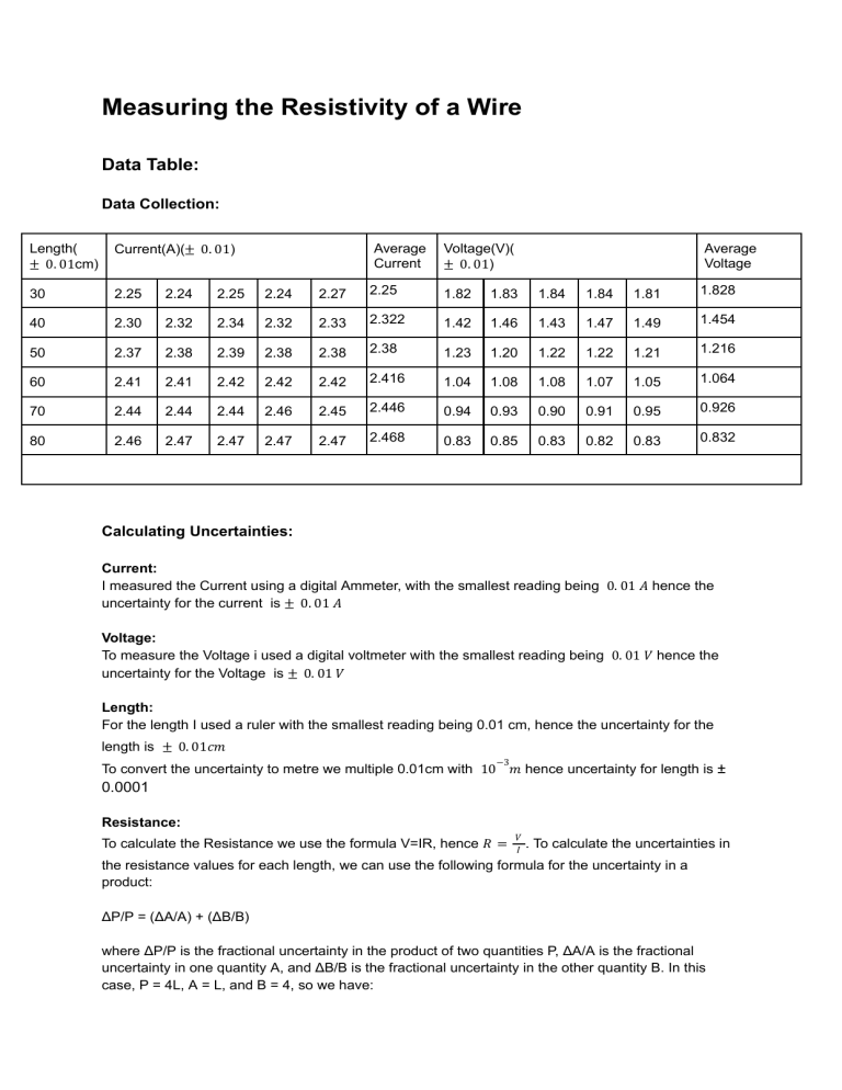
Measuring the Resistivity of a Wire
Data Table:
Data Collection:
Length(
± 0. 01cm)
Current(A)(± 0. 01)
Average
Current
Voltage(V)(
± 0. 01)
Average
Voltage
30
2.25
2.24
2.25
2.24
2.27
2.25
1.82
1.83
1.84
1.84
1.81
1.828
40
2.30
2.32
2.34
2.32
2.33
2.322
1.42
1.46
1.43
1.47
1.49
1.454
50
2.37
2.38
2.39
2.38
2.38
2.38
1.23
1.20
1.22
1.22
1.21
1.216
60
2.41
2.41
2.42
2.42
2.42
2.416
1.04
1.08
1.08
1.07
1.05
1.064
70
2.44
2.44
2.44
2.46
2.45
2.446
0.94
0.93
0.90
0.91
0.95
0.926
80
2.46
2.47
2.47
2.47
2.47
2.468
0.83
0.85
0.83
0.82
0.83
0.832
Calculating Uncertainties:
Current:
I measured the Current using a digital Ammeter, with the smallest reading being 0. 01 𝐴 hence the
uncertainty for the current is ± 0. 01 𝐴
Voltage:
To measure the Voltage i used a digital voltmeter with the smallest reading being 0. 01 𝑉 hence the
uncertainty for the Voltage is ± 0. 01 𝑉
Length:
For the length I used a ruler with the smallest reading being 0.01 cm, hence the uncertainty for the
length is ± 0. 01𝑐𝑚
−3
To convert the uncertainty to metre we multiple 0.01cm with 10 𝑚 hence uncertainty for length is ±
0.0001
Resistance:
To calculate the Resistance we use the formula V=IR, hence 𝑅 =
𝑉
𝐼
. To calculate the uncertainties in
the resistance values for each length, we can use the following formula for the uncertainty in a
product:
ΔP/P = (ΔA/A) + (ΔB/B)
where ΔP/P is the fractional uncertainty in the product of two quantities P, ΔA/A is the fractional
uncertainty in one quantity A, and ΔB/B is the fractional uncertainty in the other quantity B. In this
case, P = 4L, A = L, and B = 4, so we have:
△𝑅
𝑅
=
∆𝑉
𝑉
+
∆𝐼
𝐼
where Δ(R) is the uncertainty in resistance, ΔV is the uncertainty in voltage, and ΔI is the uncertainty
in current.
Average Uncertainties:
For calculating the average uncertainties, we use the formula:
𝑀𝑎𝑥𝑖𝑚𝑢𝑚 𝑉𝑎𝑙𝑢𝑒 − 𝑀𝑖𝑛𝑖𝑚𝑢𝑚 𝑉𝑎𝑙𝑢𝑒
2
Using the above mentioned methods, the uncertainties for the variables are as follows:
Length(m)
Length
uncertainty(
m)
Average
Current(I)
Uncertainty For
current(I)
Average
Voltage(V)
Uncertainty for
voltage(V)
0.30
± 0.0001
2.25
±0.015 1.83
±0.02
0.40
± 0.0001
2.32
±0.02 1.45
±0.04
0.50
± 0.0001
2.38
±0.01 1.22
±0.02
0.60
± 0.0001
2.42
±0.01 1.06
±0.02
0.70
± 0.0001
2.45
±0.01 0.93
±0.03
0.80
± 0.0001
2.47
±0.01 0.83
±0.02
Data Processing:
Length(±
0.0001m)
Average Current(I)
Average Voltage(V)
Resistance(Ω)
0.30
2.25
±0.015
1.828
±0.015
0.812 ± 0.012
0.40
2.322
±0.02
1.454
±0.035
0.626 ±0.020
0.50
2.38
±0.01
1.216
±0.015
0.511 ±0.008
0.60
2.416
±0.005
1.064
±0.02
0.440 ±0.009
0.70
2.446
±0.01
0.926
±0.025
0.379 ±0.0118
0.80
2.468
±0.005
0.832
±0.015
0.337 ±0.007
Data Presentation:
Graph of Resistance against length of the wire
Data Analysis:
To further Analyse my data I will use the equation 𝑅 =
ρ𝐿
𝐴
where ρ is the resistivity of the
metal wire which in this case is copper, L is the length of the wire and A is the cross
sectional Area.
𝑅=
Calculating uncertainties
ρ𝐿
𝐴
The diameter was measured using a screw
gauge, hence the zero error was 0.02mm.
Hence the diameter is 0.53mm-0.02mm which is
0.51mm. With the uncertainty being ±0.01mm.
2
Area=
1
4
× π ×𝑑
Area=
1
4
× π × (0. 51 × 10 )
−3 2
−7
Area= 2.04× 10
2
𝑚
For the experiment, The wire used was a
−8
copper wire, hence ρ is 1. 62 × 10 Ω 𝑚.
Hence for 𝑅 =
ρ𝐿
𝐴
To calculate the uncertainty of area we use the
formula for the uncertainty in a product:
ΔP/P = (ΔA/A) + (ΔB/B)
In this case it is:
△𝐴
𝐴
=(
∆𝑑
𝑑
)×2
−7
A is 2.04 × 10
2
𝑚
There is no uncertainty for π because π is a
constant.
and ρ is
−6
Hence uncertainty for Area is:
1. 77 × 10 Ω 𝑚.
−6
𝑅=
1.77 ×10
−3
△𝐴
𝐿
−7
2.04×10
−7
2.04 ×10
=(
𝑅 = 0. 87𝐿
∆𝐴 = 8 × 10
Gradient Calculations
𝑅
𝐿
Gradient= 0.87
Maximum Gradient= -0.89
Minimum gradient = -0.99
Average Gradient=
𝑀𝑎𝑥 + 𝑀𝑖𝑛
2
Average Gradient=
−0.99 + −0.89
2
Average Gradient= -0.94
Uncertainty for Gradient=
Uncertainty =
−3
(0.51×10
−9
Hence a graph of R/L should have a
gradient of 0.87.
Gradient =
0.01×10
𝑀𝑎𝑥 − 𝑀𝑖𝑛
2
−0.89 − −0.99
2
Uncertainty = ± 0. 05
Percentage Uncertainty = 5.32%
2
𝑚
)×2
Conclusion:
In conclusion, the experimental results obtained in this wire resistivity experiment were
unexpected, as they showed a decrease in resistance with an increase in the length of the
wire. The observed negative correlation between length and resistivity is inconsistent with
the theoretical understanding. However, despite the unexpected findings, the experiment
demonstrated the importance of careful measurement and analysis in scientific
investigations. It highlighted the need for accurate instruments, proper calibration, and
attention to detail. By comparing the experimental results with the known resistivity values of
the wire material, it will be possible to evaluate the accuracy of the experiment and
determine the extent of any systematic errors.
Overall, while the results of this experiment did not align with the expected outcomes, the
experiment was accurate and precise, the presence of systematic and random errors were
minimal, hence as seen in the gradient calculations the percentage error was only 5.32%.
Evaluation:
The data which showed that when resistance decreases with an increase in the length of the
wire, is unexpected based on the theoretical understanding of resistance and the equation
𝑅=
ρ𝐿
𝐴
. Normally, an increase in length should result in an increase in resistance.
During the experiment, various calculations and measurements were performed to
determine the resistivity of the wire. However, upon analysing the data, some limitations and
sources of error became apparent.
One potential source of error lies in the measurement of the wire's diameter using a screw
gauge. Although efforts were made to rotate the wire and take multiple measurements at
different points, there may still be slight variations in the recorded diameter. The uncertainty
of ±0.01mm suggests that the true diameter could fall within a small range around the
measured value. These uncertainties in diameter measurements contribute to the
uncertainty in the calculated cross-sectional area, hence reducing the accuracy of the
experiment.
Resistance is temperature-dependent, hence variations in temperature can affect the
resistance of the wire. If the wire heated up during the experiment, it could have caused a
decrease in resistance, leading to the observed results. The experiment was done in a hurry
due to time constraints, where there was constant high power supply to the wire resulting in
increasing temperature, Hence a possible extension that could have been made during the
experiment was to monitor the temperature during the experiment using a thermometer or
temperature sensor placed near the wire. Recording the temperature could allow for further
analysis and potential correction of resistance values.
The analysis of the graph depicting the relationship between resistance (R) and length (L)
revealed a significant deviation from the expected gradient of 0.87. The actual gradient
obtained from the data analysis was found to be -0.94, indicating a substantial discrepancy
between the observed results and the theoretical prediction. The uncertainty in the gradient
was determined to be 0.05, corresponding to a percentage uncertainty of 5.32%. This could
be a result of the quality or uniformity of the wire used in the experiment. Variations in wire
quality, such as inconsistencies in diameter, can introduce uncertainties in the resistance
measurements, leading to deviations in the calculated gradient. Hence an extension could
be to ensure that the wire used is of high quality with constant variables such as diameter
throughout the wire.
Furthermore, the contact resistance between the flying lead and the wire should be taken
into account. Poor or inconsistent contact can introduce additional resistance, thus affecting
the resistance measurements and ultimately influencing the calculated gradient. Ensuring
consistent contact points throughout the experiment can help minimise contact resistance.
To further understand the relationship between resistance and length, we could extend the
experiment by using wires of different materials or varying diameters. This would allow for
comparisons and analysis of how different wire properties influence the observed resistance
trends. Additionally, repeating the experiment multiple times and increasing the number of
data points could improve the reliability of the results and help identify any outliers or
inconsistencies hence decreasing random errors.
Hence, the theoretical equation 𝑅 =
ρ𝐿
𝐴
assumes an ideal scenario with uniform resistivity,
constant cross-sectional area, and negligible contact resistance. However, in practice, these
assumptions may not hold true. Deviations from ideal conditions can introduce uncertainties
and lead to deviations in the observed resistance-length relationship. Understanding the
limitations of the theoretical model and acknowledging the potential impact of these
deviations is crucial for accurate data interpretation.
In conclusion, to improve the accuracy and reliability of the experiment, it is essential to
address measurement uncertainties, assess wire quality and uniformity, consider contact
resistance, and account for temperature effects. Implementing improvements, such as
utilising more precise measurement techniques, calibrating the setup using wires with known
resistivity values, and conducting detailed error analyses, can enhance the experimental
setup and measurement techniques. These steps will ultimately lead to a better
understanding of the relationship between resistance, length, and resistivity and provide
more reliable experimental results.