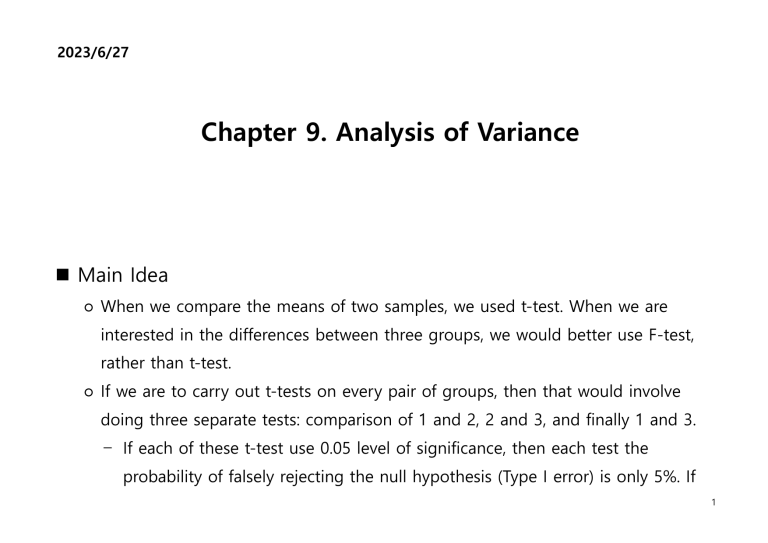
2023/6/27
Chapter 9. Analysis of Variance
 Main Idea
○ When we compare the means of two samples, we used t-test. When we are
interested in the differences between three groups, we would better use F-test,
rather than t-test.
○ If we are to carry out t-tests on every pair of groups, then that would involve
doing three separate tests: comparison of 1 and 2, 2 and 3, and finally 1 and 3.
– If each of these t-test use 0.05 level of significance, then each test the
probability of falsely rejecting the null hypothesis (Type I error) is only 5%. If
1
we assume each test is independent, then the overall probability of no Type I
error is .953 = .857.
– So, the probability of at least one Type I error is 1 - .857 = .143 or 14.3%.
○ An ANOVA produces an F-statistic, which is similar to the t-statistic in that it
compares the amount of systematic variance to the unsystematic variance.
– It tests overall effect 𝑥̅1 = 𝑥̅2 = 𝑥̅3 .
Treatment
Sample size
Sample mean
1
2
j
x11
x12
x21
.
.
.
x22
.
.
.
x2j
.
.
.
x2k
.
.
.
xn11
xn22
xnjj
xnkk
n1
𝑥̅1
n2
𝑥̅2
nj
𝑥̅𝑗
nk
𝑥̅𝑘
...
x1j
k
...
x1k
­ Xij= ith observation of jth sample.
2
­ nj = the number of observations in the same j.
­ 𝑥̅𝑗 = the mean of the jth sample.
­ 𝑥̿ = the gran mean of all the observation.
○ Test statistic
­ Sum of Squares for Model (between-treatment variation)
𝑘
SSM = ∑ 𝑛𝑗 (𝑥̅𝑗 − 𝑥̿ )2
𝑗=1
 If 𝑥̅1 = 𝑥̅2 = . . . = 𝑥̅𝑘 , then SSM=0.
­ Sum of Squares of Error (within-treatments variation)
𝑘
𝑛𝑗
SSE = ∑ ∑ 𝑛𝑗 (𝑥𝑖𝑗 − 𝑥̅𝑗 )2
𝑗=1 𝑖=1
­ Mean Squares of Model
MSM =
­ Mean Squares of Error
𝑆𝑆𝑀
𝑘−1
3
MSE =
𝑆𝑆𝐸
𝑛−𝑘
F=
𝑀𝑆𝑀
𝑀𝑆𝐸
- Test statistic
 Two types of datafile.
­ Wide type file
`Bumper 1` `Bumper 2` `Bumper 3` `Bumper 4`
1
610
404
599
272
2
354
663
426
405
3
234
521
429
197
4
399
518
621
363
5
278
499
426
297
6
358
374
414
538
7
379
562
332
181
8
548
505
460
318
9
196
375
494
412
10
444
438
637
499
­ Long type datafile
values
ind
4
1
610 Bumper 1
2
354 Bumper 1
3
234 Bumper 1
4
399 Bumper 1
5
278 Bumper 1
6
358 Bumper 1
○ R only uses long type datafile for AOV or Regression, and etc. You have to use
command “stack” and “unstack” to change the datafile types.
Ex 9-1)
A car company is considering several new types of bumpers. To test how well
they react to low-speed collisions, 10bumpers of each of four different types
were installed. The cost of repairing the damage in each case was assessed. Is
there sufficient evidence at the 5% significance level to infer that the bumpers
differ in their reactions to collision?
>
>
>
>
library(readxl)
bumper <- read_excel("R/data/22F data/Ex9-1.xlsx")
View(Ex9_1)
bumperstack <-stack (Ex9-1)
# Change into a long file.
5
> summary(aov(values~ind))
Df Sum Sq Mean Sq F value Pr(>F)
ind
3 150884
50295 4.056 0.0139 *
Residuals
36 446368
12399
--Signif. codes: 0 ‘***’ 0.001 ‘**’ 0.01 ‘*’ 0.05 ‘.’ 0.1 ‘ ’ 1
The p-value of bumper is .014 << .05. We can conclude that there exist differences
in the cost between bumpers.
Ex 9-2) Two-factor Experiment
A survey was conducted in which Americans aged between 37 and 45 were
asked how many jobs they have held in their lifetimes. Education levels are
1: Less than high school
2: High school
3: Some college without degree
4: At least one university degree.
The gender categories are: 1: male and 2: female.
6
Can we infer that differences exist between genders and educational levels?
> X14_4b <- read_excel("R/data/22F data/Ex9-2.xlsx")
> View(Ex9_2)
> twoaov <- aov(Jobs ~ Gender*Education, data= Ex9_2)
> anova (twoaov)
Analysis of Variance Table
Response: Jobs
Df Sum Sq Mean Sq F value
Pr(>F)
Gender
1 11.25 11.250 1.1655 0.2837386
Education
1 134.56 134.560 13.9406 0.0003624 ***
Gender:Education 1
0.16
0.160 0.0166 0.8978966
Residuals
76 733.58
9.652
--Signif. codes: 0 ‘***’ 0.001 ‘**’ 0.01 ‘*’ 0.05 ‘.’ 0.1 ‘ ’ 1
The p-value for Gender is .29 >> .05. There is no evidence at the 5%
significance level to infer that differences in the number of jobs exist between
men and women.
The p-value for Education is .00036 << .05. There is sufficient evidence to
conclude that differences in the number of jobs exist between educational level.
7
> twoaov1 <- aov(Jobs ~ Gender + Education, data= Ex9_2)
> anova (twoaov1)
Analysis of Variance Table
Response: Jobs
Df Sum Sq Mean Sq F value
Gender
1
11.25
11.250
Pr(>F)
1.1806 0.2806246
Education 1 134.56 134.560 14.1210 0.0003316 ***
Residuals 77 733.74
9.529
--Signif. codes: 0 ‘***’ 0.001 ‘**’ 0.01 ‘*’ 0.05 ‘.’ 0.1 ‘ ’ 1
8