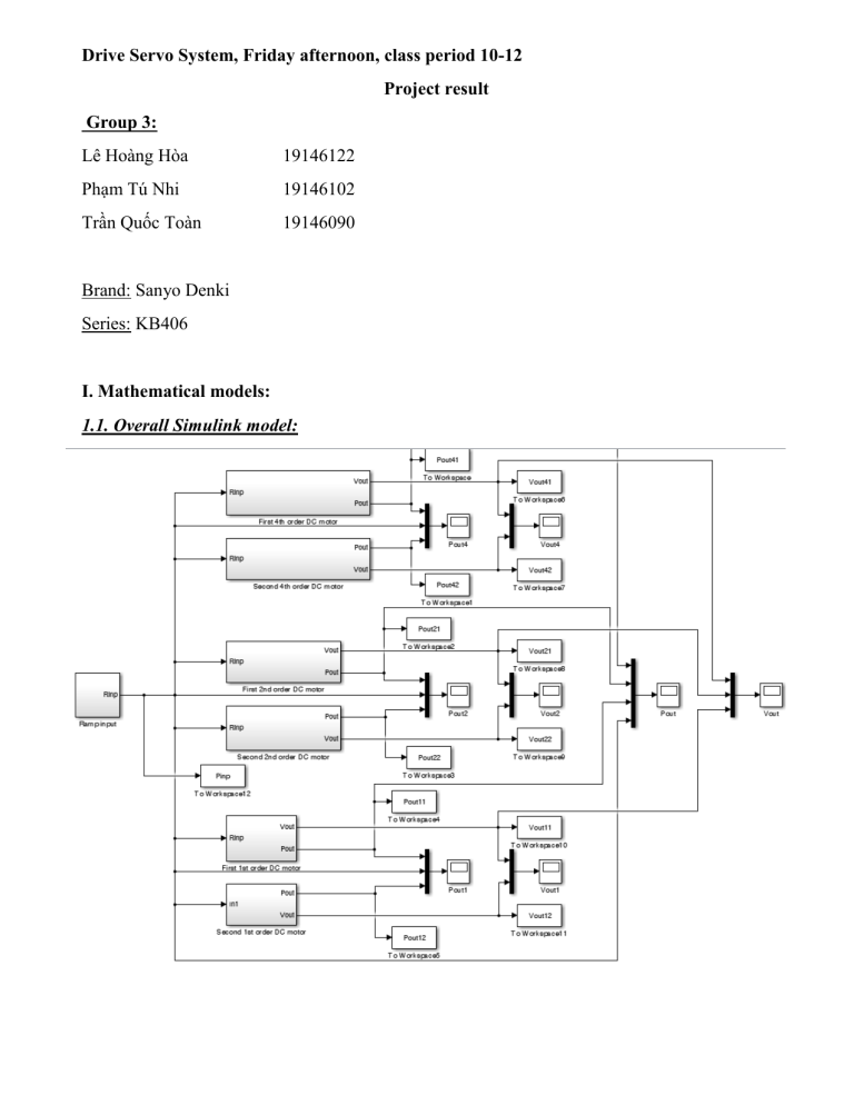
Drive Servo System, Friday afternoon, class period 10-12
Project result
Group 3:
Lê Hoàng Hòa
19146122
Phạm Tú Nhi
19146102
Trần Quốc Toàn
19146090
Brand: Sanyo Denki
Series: KB406
I. Mathematical models:
1.1. Overall Simulink model:
1.2. Ramp input model:
1.3. 4th order DC servo motor system model:
1.4. 2nd order DC servo motor system model:
1.5. 1st order DC servo motor system model:
II. The calculations to obtain the control parameters:
2.1. Constant:
Rotor inertia:
𝐽𝑀 = 0.108 ∗ 10−4 (𝑘𝑔. 𝑚2 )
Rated speed:
𝑁𝑅 = 3000 (min−1 ) = 314.16 (𝑟𝑎𝑑/𝑠)
Load 1:
𝑁𝐿 = 4;
𝜉 = 0;
Load 2:
𝑁𝐿 = 9;
𝜉 = 0.02; 𝐾𝐿 = 60
𝐾𝐿 = 40
2.2. MATLAB code to obtain the control parameters.
%%% thong so
Jm = 0.108*10^-4;
Ng = 1;
cp4 = 0.24; cv4 = 0.82;
cp2 = 0.24; cv2 = 0.96;
cp1 = 0.24;
%% NL = 4, psi = 0, KL = 40
NL = 4; psi = 0; KL = 40;
JL = NL*Ng^2*Jm;
omegaL = sqrt(KL/JL);
DL = 2*psi*sqrt(KL*JL);
%%% 4th order
Kp4 = cp4*omegaL; Kv4 = cv4*omegaL;
Kvg = Kv4*(Jm+JL/(Ng^2));
%%% 2nd order
Kp2 = cp2*omegaL; Kv2 = cv2*omegaL;
%%% 1st order
Kp1 = cp1*omegaL;
%% NL2 = 9, psi2 = 0.02, KL2 = 60
NL2 = 9; psi2 = 0.2; KL2 = 60;
JL2 = NL2*Ng^2*Jm;
omegaL2 = sqrt(KL2/JL2);
DL2 = 2*psi2*sqrt(KL2*JL2);
%%% 4th order
Kp42 = cp4*omegaL2; Kv42 = cv4*omegaL2;
Kvg2 = Kv42*(Jm+JL2/(Ng^2));
%%% 2nd order
Kp22 = cp2*omegaL2; Kv22 = cv2*omegaL2;
%%% 1st order
Kp12 = cp1*omegaL2;
III. The simulation results:
3.1. Overall results:
3.1.1. Position respone:
3.1.2. Velocity respone:
*Comment:
- The position and velocity respond gave the same results when we only take a overall look. So
from now on, we will only highlight the response result at the beginning and end.
3.1. Comparing all transfer function with a same speed (300 rad/s) and load:
3.1.1. Load 1:
3.1.2. Load 2:
*Comments:
- When the load is changed, the position reaction time between the 3 mode of speeds is much
more similar to an order from the second and first order functions, which is reasonable in terms
of order accuracy.
- When ξ = 0 for the load 1, the 4th order model reaches the estimated velocity much faster at the
beginning and the end of the position response than the 2nd and 1st order model; giving only 0.1
(s) of time error, proving that higher-order functions give higher time measurement accuracy.
- With load 2 (ξ = 0.02 ), the 4th order model get slower to get the respone value (up to 0.025
second of the respone time). The damping factor does not affect for 2nd and 1st equation so the
time respone of those the not change so much since it delay about 0.005 (s) compare to the load
1.
- 3 models are all needed 0.01-0.03sec more to reach the estimated position in the process of
position control.
Conclusion: The higher the damping factor, the more inaccurate of the respone time in the 4th
order equation is compared to other 2nd and 1st order transfer functions.
3.2. Comparing 3 transfer function with diffirent load:
3.2.1. High speed: v4 = 300 ( 62.83 ~ 314.16 (𝑟𝑎𝑑/𝑠) )
3.2.2 Middle speed: v2 = 60
( 15.7 ~ 62.83 (𝑟𝑎𝑑/𝑠) )
3.2.3 Low speed: v1 = 10 ( 0 ~ 15.7 (𝑟𝑎𝑑/𝑠) )
* Comments:
Apart from the above, our group also compared loads with only changing one parameter
(NL , ξ or K L ) and giving out a conclusion:
- When ξ = 0 and the ratio NL/KL is constant, the output result mostly becomes the same.
- Increasing NL, ξ or decreasing KL only causes a small delay of speed at the beginning =>
increasing response time, proportional with the order of transfer function. However, ξ doesn’t
affect anything in the 2nd and 1st order model.