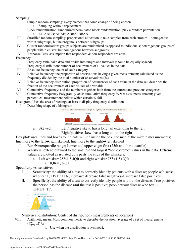
Sampling: I. Simple random sampling: every element has some change of being chosen a. Sampling without replacement II. Block randomization: randomized permutated block randomization; pick a random permutation a. Ex. AABB; ABAB; ABBA; BBAA III. Stratified random sampling: proportional allocation to take samples from each stratum—homogenous within subgroups, but heterogenous between subgroups IV. Cluster randomization: groups subjects are randomized as opposed to individuals; heterogenous groups of people within cluster, but homogenous between subgroups V. Response Bias; assumption that responders & non-responders are equal Frequency: I. Frequency table: take data and divide into ranges and intervals (should be equally spaced) II. Frequency distribution: number of occurrences of all values in the data III. Absolute frequency: count of each category IV. Relative frequency: the proportion of observations having a given measurement; calculated as the frequency divided by the total number of observations (%) V. Relative frequency distribution: proportion of occurrences of each value in the data set; describes the fraction of the occurrences of each values of a variable VI. Cumulative frequency: add the numbers together: both from the current and previous categories VII. Cumulative frequency Polygram: y-axis: cumulative frequency % & x-axis: measurement; gives percentiles: measurement bellow which certain % fall Histogram: Uses the area of rectangular bars to display frequency distribution I. Describing shape of a histogram a. Skewed: Left/negative skew: has a long tail extending to the left Right/positive skew: has a long tail to the right Box plot: uses lines and boxes to indicate w Line inside the box: the media: the middle measurements; line more to the left right skewed; line more to the right left skewed I. Box interquartile range; Lower and upper edge: first (25th and third quartile) II. Whiskers: extend outward to the smallest and largest “non-extreme” values in the data. Extreme values are plotted as isolated dots pasts the ends of the whiskers. a. Left whisker: 25th-1.5-IQR and right whisker 75th+1.5+IQR i. IQR=Q3-Q1 Specificity vs. sensitive: I. Sensitivity: the ability of a test to correctly identify patients with a disease; people w/disease who test +; TP/TP +TN; increase; decrease false negatives-> increase false positives II. Specificity: the ability of a test to correctly identify people without the disease. True positive: the person has the disease and the test is positive; people w/out disease who test -; TN/TN+TP; Numerical distribution: Center of distribution (measurements of location) VIII. Arithmetic mean: Most common metric to describe the location; average of a set of measurements = (∑𝑛𝑖=1 𝑥𝑖)/𝑛 i. Use when the distribution is symmetric This study source was downloaded by 100000759540971 from CourseHero.com on 04-26-2022 16:30:43 GMT -05:00 https://www.coursehero.com/file/95462564/Cheat-Sheetpdf/ ii. If not symmetric use: median median=50th percentile; less influenced by extreme observations; median=middle; odd: 0,1,2,3,7 median: 2; even: 0,1,2,3,5,7 median 2+3/2 IX. Geometric means: # tend to be in the powers of something; (1): take log of values; (2): take average ; (3): reverse log exponentiate; GM=10^4 X. Mode: most frequent occurring observations XI. Quick and dirty: mid-range: min+max/2 Numerical distributions: Variability of distribution (measurements of variability) about the center I. Average distance from x-bar II. Absolute distance: mean absolute deviation: = ∑𝑛𝑖=1 𝑥𝑖 − 𝑥𝑏𝑎𝑟/2; easiest way to interpret: compare to each other III. IV. Variance: square: y is x instead Standard deviation: common measure; how different measurement typically are from the mean Interpretation of s: if data comes from a normal distribution; area under 1 pt: 68% of data falls under 1S.D; 2 S.D. 95% of data falls; 3 S.D. 99.7% of data falls a. Outliers outside 3.S.D b. Don’t use if it’s not a normal distribution V. Interquartile range: use if it’s not a normal distribution(skewed); and use median b/c robust a. Median: odd: 0,1,2,3,4,7,8, 25th: 0+1+2: 1 75th: 4+7+8=7; even: 0,1,2,3,7,8 median: 2+3/2=2.5; 25th: 0+1+2/3=1 & 3,7,8/3=7 VI. Quick and dirty: range= Max-min =approx. 4S.D a. R/4=S.D Statistics and parameters: I. Statistics: anything that you can calculate on a sample: x-bar and standard deviation II. Parameter: population: mu and baby sigma a. Frequentist: imagine this experiment happening over and over III. Sampling distribution of x-bar a. Mean value: average value of this experiment=mu i. If average all x-bar, you get close to mu ii. X-bar is the unbiased estimate; can use when data is symmetric; median doesn’t have this property; is not unbiased IV. Standard deviation of the distribution a. Standard deviation of set of x-bar is sigma=standard error of x-bar uncertainty of x-bar b. Sigma reflects variation; variability depends on sample size; make clusters around mu smaller by changing V. Sampling distribution of S a. Mean of the distribution ; S is almost the average of sigma; s is approx. unbiased of sigma b. 𝑆 = √∑𝑛𝑖=1(𝑋𝑖 − 𝑥𝑏𝑎𝑟)2/(𝑛 − 1) VI. Probability: the likelihood of an event from a given statistical experiment P(E) a. Fundamental truths: axions of probabiltt; (1): 0<=P€<=1; 0=impossible b. E1, E2, E3, P(E)1+P(E)2+ P(E)3+P(E)n =1 c. Law of large numbers: P(E)=ratio as the number of experiments approaches infinity d. sampling distribution falls under this get probably from sampling distribution objective probability: subject to law of large numbers i. Subjective probability: not subject to law of large number: probability that it will rain on Monday: 40% This study source was downloaded by 100000759540971 from CourseHero.com on 04-26-2022 16:30:43 GMT -05:00 https://www.coursehero.com/file/95462564/Cheat-Sheetpdf/ Powered by TCPDF (www.tcpdf.org)


