1. Finance and Analytical Tools
Objectives: After reading this chapter, you will be able to
1. Get an overview of finance and basic algebra.
2. Use geometric series in financial calculations.
3. Understand the basic concepts of statistics.
4. Use Excel, Maple, or WolframAlpha to solve mathematical problems.
1.1
Field of Finance
When you look at the balance sheet of a company, you will see the assets and liabilities
are categorized as long-term, or short-term. In this course, we are dealing with the
management of long-term assets (machinery, equipment, buildings, land, etc.) and longterm liabilities (bonds) and other long-term financing (stocks, preferred stock). Another
course, FIN 361, Working Capital Management, deals with the management of current
assets (cash, marketable securities, accounts receivable, and inventories) and current
liabilities (accounts payable, short-term financing, and accruals).
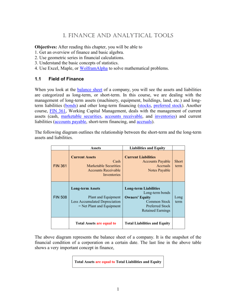
The following diagram outlines the relationship between the short-term and the long-term
assets and liabilities.
Assets
Liabilities and Equity
Current Assets
FIN 361
Cash
Marketable Securities
Accounts Receivable
Inventories
Long-term Assets
FIN 508
Plant and Equipment
Less Accumulated Depreciation
= Net Plant and Equipment
Total Assets are equal to
Current Liabilities
Accounts Payable
Accruals
Notes Payable
Short
term
Long-term Liabilities
Long-term bonds
Owners' Equity
Common Stock
Preferred Stock
Retained Earnings
Long
term
Total Liabilities and Equity
The above diagram represents the balance sheet of a company. It is the snapshot of the
financial condition of a corporation on a certain date. The last line in the above table
shows a very important concept in finance,
Total Assets are equal to Total Liabilities and Equity
1
Analytical Techniques
1. Finance and Analytical Tools
_____________________________________________________________________________
In symbols, one can write it as
V=B+S
(1.1)
In this equation,
V = total market value of the company
B = total market value of the liabilities of the company. This includes bonds and shortterm notes.
S = total market value of the stock of the company. This includes common and preferred
stock.
We will discuss this equation in more detail in chapter 9.
First, one should learn the basic financial principles, such as time value of money, risk,
options, cash flows, and the measurable quantities such as the stock price, earnings per
share, debt ratio, etc. FIN 508, explains these basic ideas, and their application to longterm financial management of a company.
You may say, “If I were a CFO of a compansy, I would monitor the spending daily.” You
will be focusing on the tan part of the diagram, which is a valid activity. You will
monitor cash, accounts receivables, inventory, and the daily cash flows. However, you
have to know the whole picture. The most important decisions are made in the blue part
of the diagram. Here you are raising and investing millions, perhaps billions, of dollars.
The recent IPO of Facebook (May 18, 2012) is a good example of this activity. If you
make an error, it may turn out to be a big mistake.
When you are making a financial decision at a company, you cannot rely entirely on gut
feeling, just because you know your business. You have to do some homework first and
find the right course of action. If you are presenting your case to a board of directors, or
in a court of law, you have to convince the audience with facts. We are learning to do that
here in this course.
The relationship between different finance courses is as follows.
→
→
MBA 503C → FIN 508 →
→
→
1.2
FIN 582 Advanced Financial Management
FIN 583 Investment Analysis
FIN 584 International Finance
FIN 585 Derivative Securities
FIN 586 Portfolio Theory
Problem Solving
One can learn finance efficiently by learning to solve financial problems analytically.
This textbook has plenty of problems, many of them are solved examples and the others
are the end-of-the-chapter exercises. There are two ways to look at any homework
problem. The first one is the quick one:
2
Analytical Techniques
1. Finance and Analytical Tools
_____________________________________________________________________________
Homework Problem → Formula → Answer
Some students have the temptation to solve the problem quickly without understanding
the concept that the problem is supposed to develop. They miss the real purpose of the
exercise, which is to consolidate an idea and observe its application.
There is another way to look at the same problem.
Is there a similar problem,
worked out in the text,
which can be applied here?
↓
Study the material in
the text to learn new
concepts
↓
Concepts, such as
risk, time value of
money, required rate
of return, options,
CAPM
→
→
Study the worked out
examples to see how the
concepts can be applied
to practical problems
↑
Can I write these
concepts in the form of
mathematical equations?
→
Homework
Problem
→
Solution
↑
Is it possible to break this
problem into a set of
simpler problems, solve
them separately, and
recombine them?
The second method is obviously more cumbersome, but it helps the student understand
the material.
Before we actually start studying finance and the financial management as a discipline, it
is worthwhile to review some of the fundamental concepts in mathematics first. This will
help us appreciate the usefulness of analytical techniques as powerful tools in financial
decision-making. We shall briefly review elementary algebra, basic concepts in statistics,
and finally learn Excel, Maple, or WolframAlpha as a handy way to cut through the
mathematical details.
Our approach toward learning finance is to translate a word problem into a mathematical
equation involving some unknown quantity, solve the equation, and get the answer. This
will help us determine an exact answer, rather than just an approximation. This will lead
to a better decision.
1.3
Video 01A, Linear Equations
To review the basic concepts of algebra, we look at the simplest equations first, the linear
equations. These equations do not have any squares, square roots, or trigonometric or
other complicated mathematical functions.
Example
1.0. Suppose John buys 300 shares of AT&T stock at $26 a share and pays a commission
of $10. When he sells the stock, he will have to pay $10 in commission again. Find the
selling price of the stock, so that after paying all transaction costs, John’s profit is $200.
3
Analytical Techniques
1. Finance and Analytical Tools
_____________________________________________________________________________
Let us define profit π as the difference between the final payoff F, after commissions, and
the initial investment I0, including commissions. We can write it as a linear equation as
follows
π = F − I0
We require a profit of $200, thus, π = 200. Suppose the final selling price of the stock per
share is x, the number we want to calculate. The initial investment in the stock, including
commission, is I0 = 300(26) + 10 = $7810. Selling 300 shares at x dollars each, and
paying a commission of $10, gives the final payoff as, F = 300x − 10. Make these
substitutions in the above equation to obtain
200 = 300x − 10 − 7810
Moving things around, we get
200 + 10 + 7810 = 300x
Or,
8020 = 300x
Or,
x = 8020/300 = 26.73333333  $26.73 ♥
This means that the stock price should rise to $26.73 to get the desired profit. Note that
the answer has a dollar sign and it is truncated to a reasonable degree of accuracy,
namely, to the nearest penny.
Next, consider a somewhat more complicated problem involving dollars, doughnuts, and
coffee.
1.1. Jane works in a coffee shop. During the first half-hour, she sold 12 cups of coffee
and 6 doughnuts, and collected $33 in sales. In the next hour, she served 17 cups of
coffee and sold 8 doughnuts, for which she received $46. Find the price of a cup of coffee
and that of a doughnut.
This is an example where we have to find the value of two unknown quantities. The
general rule is that you need two equations to find two unknowns. We have to develop
two equations by looking at the sales in the first half-hour and in the second hour.
Suppose the price of a cup of coffee is x dollars, and that of a doughnut y dollars.
First half-hour, 12 cups and 6 doughnuts for $33, gives
Second hour, 17 cups and 8 doughnuts for $46, gives
12 x + 6 y = 33
17 x + 8 y = 46
Now we have to solve the above equations for x and y.
First, try to eliminate one of the variables, say y. You can do this by multiplying the first
equation by 8 and the second one by 6, and then subtracting the second equation from the
first. This gives
8*12 x + 8*6 y = 8*33
6*17 x + 6*8 y = 6*46
4
Analytical Techniques
1. Finance and Analytical Tools
_____________________________________________________________________________
Subtracting second from first, (8*12 – 6*17) x = 8*33 – 6*46
Simplifying it,
– 6 x = – 12,
or
x=2♥
Substituting this value of x in the first equation, we have 12*2 + 6 y = 33
6y = 33 – 24 = 9
Or,
y = 9/6 = 3/2 ♥
The answer is that a cup of coffee sells for $2 and a doughnut for $1.50.
1.3
WolframAlpha
Mathematica is a useful analytical software, which has capabilities similar to Maple. It
can perform all the mathematical problems equally well. Mathematica has a website at
WolframAlpha, which is free to use. The instructions at WolframAlpha are almost
identical to those in Maple. You should explore this website and use it when you do not
have access to Maple. In this text, you can access WolframAlpha by clicking on this
button WRA.
For instance, to solve the equations in example 1.1
12 x + 6 y = 33
17 x + 8 y = 46
for x and y, enter the instructions as follows:
WRA solve(12*x+6*y=33,17*x+8*y=46)
It provides the solution as x = 2, y = 3/2.
To see the sine wave of Figure 1.1, write
WRA plot(sin(x), x=0..2*Pi)
5
Analytical Techniques
1. Finance and Analytical Tools
_____________________________________________________________________________
1.2
Non-linear Equations
Non-linear equations contain higher powers of the unknown variable, or the variable
itself may show up in the power of a number. For instance, a quadratic equation is a nonlinear equation. The general form of a quadratic equation is
ax2 + bx + c = 0
(1.2)
− b  b2 − 4ac
x=
2a
(1.3)
The roots of this equation are
Consider the following examples of non-linear equations.
Examples
1.113x = 2.678
1.2. Solve for x:
First, we recall the basic property of logarithm functions, namely,
ln(ax) = x ln a
Taking the logarithm on both sides of the given equation, we obtain
x ln(1.113) = ln(2.678)
Or,
ln(2.678) 0.9850702
x = ln(1.113) = 0.1070591 = 9.201 ♥
You can save some time by doing the calculation at WolframAlpha as follows:
WRA 1.113^x = 2.678
(2 + x)2.11 = 16.55
1.3. Solve for x,
2 + x = (16.55)1/2.11
This gives
Or,
x = (16.55)1/2.11 – 2 = 1.781 ♥
You can verify the answer at WolframAlpha as follows:
WRA (2+x)^2.11=16.55
1.4. Find the roots of
5x2 + 6x − 11 = 0
6
Analytical Techniques
1. Finance and Analytical Tools
_____________________________________________________________________________
This is a typical quadratic equation. Use equation (1.2) and put a = 5, b = 6, and c = – 11.
This gives
–6  36 – 4(5)(–11) –6  256 –6  16
11
x=
=
= 10 = − 5 or 1 ♥
10
10
You can verify the answer at WolframAlpha as follows:
WRA 5*x^2+6*x-11=0
1.3
Geometric Series
In many financial management problems, we have to deal with a series of cash flows.
When we look at the present value, or the future value, of these cash flows, the resulting
series is a geometric series. Thus, geometric series will play an important role in
managing money. Let us consider a series of numbers represented by the following
sequence
a , ax , ax2 , ax3 , ... , axn−1
The sequence has the property that each number is multiplied by x to generate the next
number in the list. There are altogether n terms in this series, the first one has no x, the
second one has an x, and the third one has x2. By this reasoning, we know that the nth
term must have xn1 in it. This type of series is called a geometric series. Our concern is
to find the sum of such a series having n terms with the general form
S = a + ax + ax2 + ax3 + ... + axn−1
(1.4)
To evaluate the sum, proceed as follows. Multiply each term by x and write the terms on
the right side of the equation one-step to the right of their original position. We can set up
the original and the new series as follows:
S = a + ax + ax2 + ax3 + ... + axn−1
xS =
ax + ax2 + ax3 + ... + axn−1 + axn
If we subtract the second equation from the first one, most of the terms will cancel out,
and we get
S − xS = a − axn
Or,
or,
S(1 − x) = a(1 − xn)
Sn =
a (1 − xn)
1−x
(1.5)
This is the general expression for the summation of a geometric series with n terms, the
first term being a, and the ratio between the terms being x. This is a useful formula,
which we can use for the summation of an annuity.
7
Analytical Techniques
1. Finance and Analytical Tools
_____________________________________________________________________________
If the number of terms in an annuity is infinite, it becomes a perpetuity. To find the sum
of an infinite series, we note that when n approaches infinity, xn = 0 for x < 1. Thus, the
sum for an infinite geometric series becomes
a
S∞ = 1 − x
(1.6)
To obtain equations (1.4) and (1.5) at WolframAlpha, use the following instructions:
WRA sum(a*x^i,i=0..n-1)
WRA sum(a*x^i,i=0..infinity)
Examples
1.5. Find the sum of
3 + 6 + 12 + 24 ..., 13 terms
We identify a = 3, x = 2, and n = 13. Putting these in (1.4), we get
a (1 − xn) 3 (1 – 213)
S = 1 − x = 1 – 2 = 3(213 – 1) = 24,573 ♥
To verify the answer at WolframAlpha, use the following instruction:
WRA sum(3*2^i,i=0..12)
1.6. Find the sum of 1.7 + 2.21 + 2.873 ..., 11 terms
Here a = 1.7, and x = 2.21/1.7 = 1.3. Also, n = 11. This gives
S=
a (1 − xn) 1.7 (1 – 1.311) 1.7(1.311 – 1)
= 1.3 − 1
= 95.89 ♥
1−x =
1 – 1.3
At WolframAlpha, use the following instruction.
WRA sum(1.7*1.3^i,i=0..10)
100 25
1.7. Find the value of  1.12i
i=1
The mathematical expression possibly means a sum of one hundred annual payments of
$25 each, discounted at the rate of 12% per annum. Write it as
100
25
25
25
25
25
25
 1.12i = 1.12 + 1.122 + 1.123 + 1.124 + ... + 1.12100
i=1
8
Analytical Techniques
1. Finance and Analytical Tools
_____________________________________________________________________________
25
This is a geometric series, with the initial term a = 1.12 , the multiplicative factor x =
1
1.12 , and the number of terms, n = 100. Use the equation
Sn =
to get
a (1 − xn)
1−x
(1.5)
(25/1.12) (1 − 1/1.12100)
Sn =
= 208.33 ♥
1 − 1/1.12
The keystrokes needed to perform the calculation on a TI-30X calculator are as follows:
25 1.12 1 1 1.12  100  1  1  1.12 
To verify at WolframAlpha, use the following instruction,
WRA sum(25/1.12^i,i=1..100)
1.4
Video 01B Elements of Statistics
Probability theory plays an important role in financial planning, forecasting, and control.
At this point, we shall briefly review some of the basic concepts of probability and
statistics. In many instances, we have to deal with quantities that are not known with
certainty. For example, what is the price of IBM stock next year or the temperature in
Scranton tomorrow? The future is unpredictable. The market may go up tomorrow, or
down. One way to get a handle on the unknown is to describe it in terms of probabilities.
For instance, there is a 30% chance that it may rain tomorrow. On the other hand, there is
an even chance that the market may go up or down on a given day. The sum of the
probabilities for all possible outcomes is, of course, one.
We may base the probabilities of different outcomes on the past observations of a certain
event. For instance, we look at the stock market for the last 300 trading days and we
notice that on 156 days it went up. Then it is fair to say that it has a 156/300 = 0.52 =
52% chance that it may go up tomorrow as well. A complete set of all probabilities is a
probability distribution. The probability distribution for the stock market may look like
this:
Outcome
Probability
Market moves up
52%
Market moves down
48%
In the above case, we are assuming that the market does not end up exactly at the closing
level of the previous day.
9
Analytical Techniques
1. Finance and Analytical Tools
_____________________________________________________________________________
The distribution in the previous example is a discrete probability distribution. Another
example of such a distribution is the set of probabilities for the outcomes of a roll of dice.
With a single die, the probability is 1/6 each of getting a 1, or 2, or 3, and so on.
A probability distribution may be continuous, such as the normal probability distribution.
The probability distribution describing the life expectancy of human beings, or machines,
is a continuous distribution. At present, we shall try to describe the uncertainty in terms
of discrete probability. We are going to use a subjective probability distribution to
describe the uncertain future.
We can find the expected value of a certain quantity by multiplying the probability of
each outcome by the value of that outcome.
Example
1.8. A project has the following expected cash flows
State of the Economy
Good
Fair
Poor
Probability
60%
30%
10%
Cash Flow X
$10,000
$6,000
$2,000
To find the expected cash flow, we compute
E(X) = .6($10,000) + .3($6,000) + .1($2,000) = $8,000
Consider a random variable X. Its outcome is X1 with a probability P1, X2 with a
probability P2, and so on. In general, the outcome is Xi with a probability Pi. Then the
expected value of X is
E(X) = P1X1 + P2X2 + ... + PiXi
Write this as
n
—
Expected value of X,
E(X) =  PiXi = X
(1.7)
i=1
Next, we would like to know how much scatter, or dispersion, is present in this expected
value of X. We may estimate this by the variance of X, or the standard deviation of X,
defining them as follows.
n
—
Variance of X,
var(X) =  Pi(Xi − X )2
(1.8)
i=1
Standard deviation of X,
σ(X) = var(X)
In the above example the standard deviation of the cash flow is
σ(X) = .6(10,000 − 8000)2 + .3(6000 − 8000)2 + .1(2000 − 8000)2 = $2683
10
(1.9)
Analytical Techniques
1. Finance and Analytical Tools
_____________________________________________________________________________
This figure represents the uncertainty, or the margin of error, in the cash flow.
At times, it is necessary to find the mutual dependence of two different events. For
example, we start two separate projects X and Y. The following table shows their
expected cash flows. The first project X, is the same as the one discussed above on the
previous page.
State of the Economy
Good
Fair
Poor
Probability
60%
30%
10%
Cash Flow X
$10,000
$6,000
$2,000
Cash Flow Y
$12,000
$8,000
$6,000
The two projects seem to be in step, both making more money in good economy and less
in poor economy. They seem to be closely related. Is there a way to measure it
quantitatively? The answer is yes, by using a measure called the correlation coefficient.
First we define the covariance between two random variables X and Y as the
n
—
—
Covariance between X and Y, cov(X,Y) =  Pi(Xi − X )(Yi − Y )
(1.10)
i=1
To find the covariance between the two projects, we must first find the expected value of
Y. Do it as
—
Y = .6($12,000) + .3($8,000) + .1($6,000) = $10,200
Next, we find
cov(X,Y) = .6(10,000  8000)(12,000  10,200)
+ .3(6,000  8,000)(8,000  10,200) + .1(2,000  8,000)(6,000  10,200)
= 6,000,000
The six-million figure found above is not particularly meaningful. We next introduce a
more practical measure of interdependence of two projects, the correlation coefficient,
defined as
cov(X,Y)
r(X,Y) = σ(X)σ(Y)
(1.11)
Write the above equation as
cov(X,Y) = r(X,Y)σ(X)σ(Y)
(1.12)
We already know (X) to be $2683. We also evaluate (Y) to be
σ(Y) = .6(12,000 − 10,200)2 + .3(8000 − 10,200)2 + .1(6000 − 10,200)2 = $2272
The smaller value of (Y) indicates that the cash flows are more tightly bunched. Finally,
we find the correlation coefficient as
cov(X,Y) 6‚000‚000
r(X,Y) = σ(X)σ(Y) = 2683*2272 = .9843 ♥
11
Analytical Techniques
1. Finance and Analytical Tools
_____________________________________________________________________________
Note that r(X,Y) is a pure number and its value always lies between +1 and −1. That is

−1 < r(X,Y) < 1
(1.13)
If the two projects are completely (meaning 100%), positively (meaning, moving in the
same direction) correlated, the correlation coefficient between them is +1. This will be
the case if one project is a carbon copy of the other one. If they are totally unrelated, the
coefficient should be 0. This will be the case if one project is completely independent of
the other one. If the two projects are such that whatever happens in one, the exact
opposite happens with the other, then their correlation coefficient is −1.
The high value of r(X,Y), .9843, in the above example is not particularly surprising
because the two projects go hand in hand, performing well in good times and poorly in
bad times. Some of these ideas are particularly helpful in understanding the risk and
return of different portfolios.
1.5
Excel
It is important that the students are able to set up finance problems using Excel, which is
now a standard of business and industry. A good working knowledge of this software
should be an integral part of every business student’s education. Almost all business
programs offer courses in the use of this software. If you want to brush up your skill in
the use of Excel, you may go the following Microsoft website for a variety of tutorials.
http://office.microsoft.com/en-us/training/CR100479681033.aspx
To get started on Excel, consider one of the previous problems that we solved by using
the logarithm function.
1.113x = 2.678
1.2. Solve for x:
Set up the table shown below. Adjust the number in the green cell B2 until the numbers
in cells B3 and B4 come very close together. B2 gives the answer.
1
2
3
4
A
Base =
Unknown power =
Result (given) =
Result(calculated) =
B
1.113
9.201184226
2.678
=B1^B2
It is possible to embed an Excel table within a Word document. To do that, go the Insert
tab in a Word document. When it opens, click on Table. In the Table menu, click on
Excel Spreadsheet near the bottom. An Excel sheet opens up, where you can do your
work. When you finish your Excel work, click anywhere on the Word document, and you
can leave Excel. To go back into the Excel spreadsheet, double-click on the table, which
will reveal all the calculations and formulas.
12
Analytical Techniques
1. Finance and Analytical Tools
_____________________________________________________________________________
Next, consider example 1.8 on page 8 again. Set it up on Excel as follows.
A
State of the Economy
Good
Fair
Poor
E(X)
E(Y)
Cov(X,Y)
sigma(X)
sigma(Y)
r(X,Y)
1
2
3
4
5
6
7
8
9
10
B
Probability
60%
30%
10%
=B2*C2+B3*C3+B4*C4
=B2*D2+B3*D3+B4*D4
=B2*(C2-B5)*(D2-B6)+B3*(C3-B5)*(D3-B6)+B4*(C4-B5)*(D4-B6)
=SQRT(B2*(C2-B5)^2+B3*(C3-B5)^2+B4*(C4-B5)^2)
=SQRT(B2*(D2-B6)^2+B3*(D3-B6)^2+B4*(D4-B6)^2)
=B7/B8/B9
C
Cash Flow X
10000
6000
2000
8000
10200
6000000
2683.28157
2271.56334
0.98437404
D
Cash Flow Y
12000
8000
6000
The numerical results of the formulas in cells B5:B10 are given in green cells C5:C10.
The principal advantage of Excel is that it can handle large tables of numbers.
1.6
Video 01C Maple
Maple is an extremely powerful analytical software. Working with Maple is quite easy.
The help facility in Maple is very valuable and it can guide the user through various
steps, using plenty of examples. Maple has extensive application in science, mathematics,
engineering, and finance. Time spent in learning this program can pay rich dividends in
terms of greater accuracy and higher productivity. The following instructions will get you
started with Maple.
Since Maple interprets capital and lower case letters distinctly, we should use the
symbols carefully. Maple has many built in mathematical functions and constants, such
as
ln, exp, Pi, sin, sqrt
Maple can do exact arithmetic calculations and displays the answer in its totality. For
example, we need the exact value of 264, or the factorial of 50, or the value of  to 50
significant figures. We do this as follows: enter the commands at the > prompt, end each
line with a semicolon, and strike the return key.
2^64;
18446744073709551616
50!;
30414093201713378043612608166064768844377641568960512000000000000
evalf(Pi,50);
3.1415926535897932384626433832795028841971693993751
Here
evalf
13
Analytical Techniques
1. Finance and Analytical Tools
_____________________________________________________________________________
calculates the result in floating point with 50 significant figures. Maple can also do
algebraic calculations. For instance, to solve the equations
5x + 6y = 7
6x + 7y = 8
for x and y, enter the instructions as follows:
eq1:=5*x+6*y=7;
eq1 := 5 x + 6 y = 7
eq2:=6*x+7*y=8;
eq2 := 6 x + 7 y = 8
solve({eq1,eq2},{x,y});
{y = 2, x = -1}
The symbol := is used specifically to define objects in Maple. In other words, if we type
eq1;
then the computer will recall the equation defined as eq1 and display it as
5x+6y=7
Maple can also do differentiation and integration. Consider the function
ln x
x3 + x
To differentiate this function with respect to x, we type in
diff(x^3+ln(x)/x,x);
1 ln(x)
3 x2 + x2 − x2
To integrate the result with respect to x, recreating the original function, we enter
int(%,x);
ln x
x3 + x
Here we use % as a symbol to designate the previous expression.
We can also use Maple to plot functions. For instance, if we want to see the visual
representation of the well-known sine wave, as in Figure 1.1, we write.
14
Analytical Techniques
1. Finance and Analytical Tools
_____________________________________________________________________________
plot(sin(x),x=0..2*Pi);
Fig. 1.1: Plot of sin x for 0 < x < 2
It is possible to add text in the plots, draw three-dimensional or animated plots, and draw
plots in color. All plots in this book are drawn with the help of Maple.
Problems
Solve the following equations:
1.9.
16x – 54 = 15x – 32
x = 22 ♥
1.10. (x +1) (x − 2) = (x – 1) (x + 2)
x=0♥
1.11. (10 x + 3) (3 x + 4) = (5 x + 6) (6 x + 7)
x = −15/11 ♥
x–2 x–7
1.12. x – 3 = x – 9
x = –3 ♥
x+4 x+6
1.13. x + 5 = x + 8
x = –2 ♥
Solve the following equations for x and y:
1.14.
1.15.
2x + 6y = 32
5x + 8y = 45
x = 1, y = 5 ♥
3x + 4y = 15
5x + 8y = 45
x = –15, y = 15 ♥
1.16. At Wal-Mart, in the hardware department, a customer buys five gallons of paint
and six brushes and pays $97.52 for them, including 6% sales tax. Another person buys
eight gallons of paint and five brushes and pays $146.28, including the sales tax. Find the
price of a gallon of paint and that of a brush.
Paint, $16 per gallon; brushes, $2 each ♥
15
Analytical Techniques
1. Finance and Analytical Tools
_____________________________________________________________________________
Solve for x,
1.17.
(1 + x)3.2 = 8.4
x = 0.9446 ♥
1.18.
1.767x = 3.876
x = 2.38 ♥
1.19.
3.909x = 15.99
x = 2.033 ♥
1.20.
2x2 + 7x – 9 = 0
x = 1, –9/2 ♥
1.21.
3x2 + 4x – 7 = 0
x = 1, –7/3 ♥
1.22. 2.5 + (2.5)(.3) + (2.5)(.3)(.3) ..., infinite terms
3.571 ♥
1
1
1
1.23. 1.1 + 1.12 + 1.13 + ... 9 terms
5.759 ♥
Find the roots of
Find the sum of the following series:
30 30(1.05) 30(1.05)2
1.24. 1.12 + 1.122 + 1.123 + ... 36 terms
386.60 ♥
10 500
1.25.  1.12i
i=1
2825.11 ♥
100 25
1.26.  1.12i
i=1
208.33 ♥
24 300
1.27. Write WolframAlpha instruction to find the sum,  1.01i
i=1
sum(300/1.01^i,i=1..24), 6373.02 ♥
1.28. The cash flows from two projects under different states of the economy are as
follows:
State of the economy Probability Project A Project B
Poor
20%
$3000
$5000
Average
30%
$4000
$7000
Good
50%
$6000
$15,000
Find the coefficient of correlation between the two projects.
.9922 ♥
1.29. The expected return from two stocks, Microsoft and Boeing, under different states
of the economy are as follows:
16
Analytical Techniques
1. Finance and Analytical Tools
_____________________________________________________________________________
State of the economy Probability Microsoft Boeing
Poor
10%
−5%
−40%
Average
40%
10%
−10%
Good
50%
20%
50%
(A) Find the expected return of Microsoft and of Boeing.
(B) Find the σ of Microsoft and of Boeing.
(C) Find the coefficient of correlation between the two stocks.
13.5%, 17% ♥
7.762%, 34.07% ♥
.9471 ♥
Key Terms
Accounts payable, 1
Accounts receivable, 1
Accruals, 1
annuity, 7
Cash, 1
Common stock, 1
correlation coefficient, 10, 11
covariance, 10
Excel, 1, 3, 11, 12
expected value, 9, 10
geometric series, 1, 6, 7
Inventories, 1
linear equation, 1
linear equations, 3, 5
Long-term bonds, 1
Maple, 1, 3, 12, 13, 14
Marketable securities, 1
normal probability
distribution, 9
Notes payable, 1
17
perpetuity, 7
Preferred stock, 1
probability distribution, 9
quadratic equation, 1, 5
Retained earnings, 1
standard deviation, 10
statistics, 1, 3, 8