LAB 1: MATLAB - Introduction to Programming
Objective:
The objective of this laboratory is to review how to use MATLAB as a programming tool and to
review a classic analytical solution to a steady-state two-dimensional heat transfer conduction
problem. We will also review how to write a program that is well documented and easy to read.
Background:
The steady-state two-dimensional temperature distribution, T(x, y), in a solid with constant
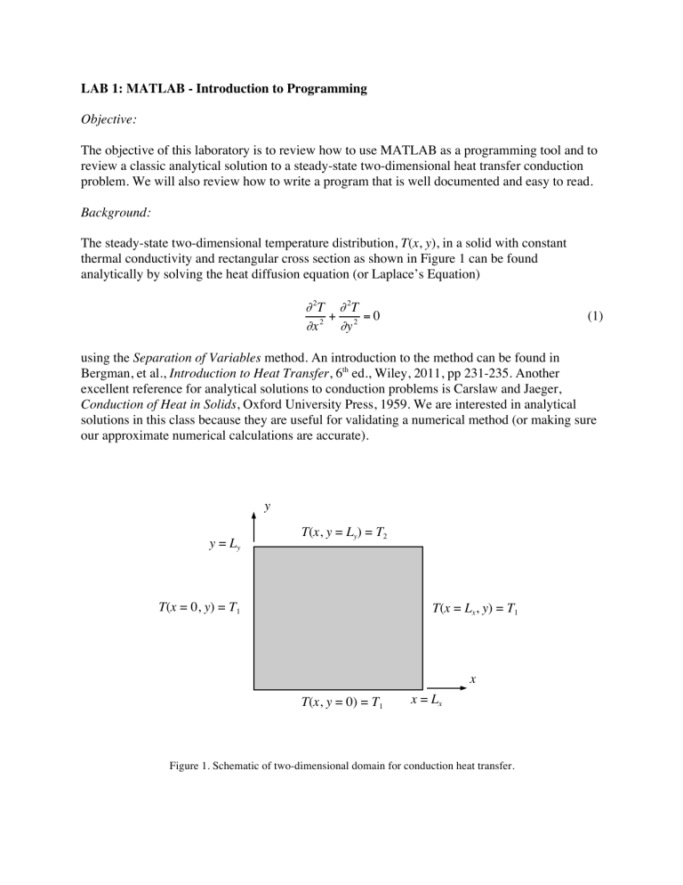
thermal conductivity and rectangular cross section as shown in Figure 1 can be found
analytically by solving the heat diffusion equation (or Laplace’s Equation)
∂ 2T ∂ 2T
+
=0
∂x 2 ∂y 2
(1)
using the Separation of Variables method. An introduction to the method can be found in
Bergman, et al., Introduction to Heat Transfer, 6th ed., Wiley, 2011, pp 231-235. Another
€ solutions to conduction problems is Carslaw and Jaeger,
excellent reference for analytical
Conduction of Heat in Solids, Oxford University Press, 1959. We are interested in analytical
solutions in this class because they are useful for validating a numerical method (or making sure
our approximate numerical calculations are accurate).
y
y = Ly
T(x, y = Ly) = T2
T(x = 0, y) = T1
T(x = Lx, y) = T1
x
T(x, y = 0) = T1
x = Lx
Figure 1. Schematic of two-dimensional domain for conduction heat transfer.
As an example, for the following boundary conditions shown in Figure 1
T ( x = 0, y ) = T1, T ( x = Lx , y ) = T1, T ( x, y = 0) = T1, T ( x, y = Ly ) = T2
(2)
where T1 and T2 are constant temperatures and dimensionless temperature θ ( x, y ) is defined as
€
€
€
€
T ( x, y ) − T1
θ ( x, y ) =
T2 − T1
(3)
€
the analytical solution can be determined to be
€
2
θ ( x, y ) =
π
∞
∑
n=1
(−1)
n +1
n
+1
% n π x ( sinh( n π y Lx )
sin'
.
*
& Lx ) sinh( n π Ly Lx )
(4)
which is an infinite series solution.
Laboratory:€
For this laboratory, you will write a MATLAB m-file to calculate the temperature from the
analytical solution above at a matrix of x and y coordinates and make a contour plot of the
results. Below are some general instructions on how to write your program. Please refer to the
online MATLAB help files as needed for more complete information. If you have not previously
used MATLAB, or if you have forgotten some of MATLAB’s features or syntax, you should use
the program help material before starting this assignment. In particular, use the “Help” menu
item and “Product Help” sub menu item to bring up the “Help” window. On the left press the
“Contents” tab. Under the “MATLAB” and “Getting Started” submenus read through the
material in the “Quick Start,” “Language Fundamentals,” “Mathematics,” “Graphics,” and
“Programming” sections.
1. Open MATLAB by double clicking on the MATLAB icon on the desktop. Create a new script
(or m-file) using the “File”, “New”, and “Script” menu item. Save the file as “ME554_lab1.m”
(or anything else, but do NOT use a name with spaces) using the “File” and “Save As” menu
item. Recall that a script (or m-file) is simply a list of MATLAB instructions saved in a file with
a “.m” extension. Write a header for your program using “%” for comment lines. Your header
should include the program name, description, your name, date created, date last modified, and a
variable list with definitions (come back and add these later). Continue to use many comment
lines throughout your program to describe each subsequent set of commands and to indicate units
for each parameter.
2. Next, put a line with just
clear, clc
to clear the memory of all variables and clear the screen.
2
3. Set the values for the geometry and boundary condition parameters (Lx, Ly, T1, and T2). You
can do this generally in three ways: simple assignment statement, by reading input from the
screen during execution, or by reading data from a file. Use the first method for some of the
input as follows:
T1 = 100; % deg. Celsius
where the semicolon suppresses output during execution and the units are included as a
comment. Also, try using the second method with an input statement:
T2 = input(‘Input temperature at y = Ly in deg. C:
‘)
4. Create vectors of x and y values of the coordinates at which you need to evaluate the
temperature. First, set Nx and Ny to the number of increments in each direction. Again, you can
do this with any of the methods given is Step 2. Second, calculate the increments between
calculations:
dx = Lx/Nx;
dy = Ly/Ny;
% m, increment in x-direction
% m, increment in y-direction
Third, create the vectors of x and y values using the following:
x = [0:dx:Lx];
y = [0:dy:Ly];
If you do not know what these lines create, enter them in the “Command Window” in MATLAB
with numbers substituted for the variables to test their output. Note that these lines demonstrate
some of the power of MATLAB in that you can create a vector of data in a single line, unlike
FORTRAN or c++.
5. Initialize a matrix to store the data for θ during calculations using the zeros function and set
θ = 1 at your top boundary using:
€
theta = zeros(Nx + 1, Ny + 1);
theta(:,Ny+1) = 1;
This is required for two reasons: (1) to allocate the correct amount of space in memory for your
array and (2) to initialize θ to zero for the summation in the next step.
6. Calculate the value of θ at each (x, y) location. To do this, use two nested for loops to cycle
through each (x, y) location with the following syntax:
for j = 2:Ny
for i = 2:Nx
% insert Equation (4) here
end
end
3
You will need to use a third nested for loop to sum up the terms in Equation (4). Use “…” to
continue your equation on the next line to make it easier to read. Note that for MATLAB “pi”
will give you π with sufficient precision. For this sum, let n go from 1 to 199. Because you are
stopping the calculation at a finite number of terms your results will have truncation error in
addition to machine precision error for double precision calculations. Note that in Equation (4),
for even values of n, the summation term goes to 0 so you can skip these terms to speed up the
calculation. One way to do this in MATLAB is to use “for n = 1:2:199” which increments
n by 2 for each loop instead of the default increment of 1.
7. Convert the calculated θ matrix to temperatures using the variable name “T”.
8. Print out temperature data to the screen for review using fprintf to produce formatted
output. The following lines work well:
for j = Ny+1:-1:1
fprintf('%7.1f', T(:,j))
fprintf('\n')
end
These lines print out the temperatures in the order you would expect for a Cartesian coordinate
system (rotated counterclockwise 90˚ as shown in Figure 2). The ‘%7.1f’ sets the format for the
temperatures as floating point with seven spaces and one number after the decimal place. The
‘\n’ adds a carriage return between lines. Alternatively, you can use (fliplr(T))’ or
rot90(T) to rotate the T matrix before printing it out.
9. Make a contour plot of the resulting temperatures using the following lines:
dT = (T2 – T1)/Nc;
v = T1:dT:T2;
colormap(jet)
contourf(x, y, T', v)
colorbar
Tmax = max(T1, T2)
Tmin = min(T1, T2)
caxis ([Tmin, Tmax])
axis equal tight
title('Contour Plot of Temperature in deg. C')
xlabel('x (m)')
ylabel('y (m)')
where Nc is the number of contours (whose value needs to be set), dT is the step in temperature
between contours, and v is a vector that sets the temperature levels for the contours. The
MATLAB built in function colormap sets the colors used for contours, contourf creates the
filled contour plot where ' after T transposes the matrix, colorbar adds a scale to the plot
where caxis sets the limits, axis equal makes the x and y axes have the same length, and
xlabel and ylabel add x-axis and y-axis labels to the plot.
4
10. Try changing the variables or options for Steps 8 and 9 to alter the output. You can also
explore some of the many other options for plotting data. For example, changing the 4th line to
contourf(x, y, T', v, 'LineStyle', 'none')
will remove the lines between the contours.
Assignment
Submit your lab assignment as a single pdf file using PolyLearn with the items listed below.
1. Set the following values in your code: Lx = Ly = 1 m, T1 = 0 ˚C, and T2 = 100˚C. Include tables
for temperature values at each location for Nx = Ny = 5 and Nx = Ny = 10.
• Label them “Table 1” and “Table 2” along with a descriptive caption above the table.
• Include x and y locations for each temperature on your table so you can determine which
temperatures are evaluated at the same location.
• Use 4 decimal places for temperature data evaluated using double precision.
2. Verify that your solution has converged to at least four decimal places for temperatures on the
interior of your domain. Discuss how limits in machine precision and truncating the infinite
series solution to a finite number of terms influence the accuracy (be quantitative) of your
calculated temperatures. To help you answer this question use the MATLAB function eps() to
determine the accuracy of both double and single precision floating point calculations and
compare this to the magnitude of terms in your summation.
3. Compare the values in Table 1 and 2 for each case at the same coordinate locations. Are the
temperatures the same or different (be quantitative) at each location where they overlap? Briefly
explain why this result makes sense.
4. Include contour plots for the two cases in step 2. For each figure include “Figure 1” and
“Figure 2” along with a descriptive caption below the figure. Make sure that if you plot or print
out your results in grayscale that you use “grayscale” for your colormap so that each temperature
has a distinct shade.
5. Do the contour plots change for these two cases? Briefly explain why this result makes sense
and how this corresponds to the accuracy of your solution.
6. Include a copy of your final m-file.
5
Cartesian Coordinates:
Ti, j = T(x i , y j )
y
€
where
and
and
Δx = Lx N x
Δy = Ly N y
€
€
∆y
€
x i = (i −1) Δx
y j = ( j −1) Δy
€
T1, Ny+1
TNx+1, Ny+1
Figure is
shown with
Nx = Ny = 3
Ly
∆x
T1,2
T2,2
T1,1
T2,1
TNx+1, 1
x
Lx
Matrix Notation:
" T1,1
T1,2 ! T1,N y +1 %
$
'
T2,1 T2,2
" '
$
[T ] = $ "
#
" '
$
'
#TN x +1,1 ! ! TN x +1,N y +1&
€
j (column number)
NOTE: The T matrix is rotated
clockwise 90˚ relative to the
Cartesian coordinate system.
i (row number)
Figure 2. Schematic diagrams of Cartesian coordinate system and matrix notation.
6