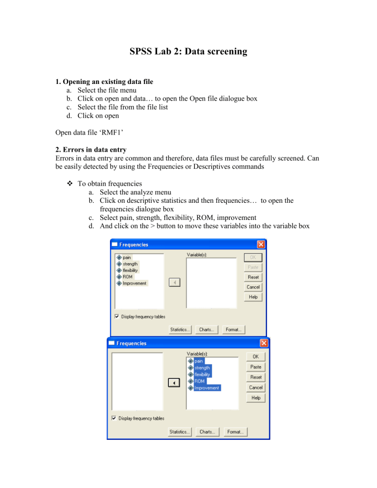
SPSS Lab 2: Data screening
1. Opening an existing data file
a. Select the file menu
b. Click on open and data… to open the Open file dialogue box
c. Select the file from the file list
d. Click on open
Open data file ‘RMF1’
2. Errors in data entry
Errors in data entry are common and therefore, data files must be carefully screened. Can
be easily detected by using the Frequencies or Descriptives commands
 To obtain frequencies
a. Select the analyze menu
b. Click on descriptive statistics and then frequencies… to open the
frequencies dialogue box
c. Select pain, strength, flexibility, ROM, improvement
d. And click on the > button to move these variables into the variable box
Frequencies
Statistics
pain
N
Valid
Missing
22
0
strengt h
22
0
flexibility
22
0
ROM
22
0
Improvement
22
0
Frequency Table
pa in
Valid
2.00
3.00
4.00
5.00
6.00
7.00
8.00
Total
Frequency
3
4
3
2
5
4
1
22
Percent
13.6
18.2
13.6
9.1
22.7
18.2
4.5
100.0
Valid Percent
13.6
18.2
13.6
9.1
22.7
18.2
4.5
100.0
Cumulative
Percent
13.6
31.8
45.5
54.5
77.3
95.5
100.0
strength
Valid
4.00
5.00
6.00
7.00
8.00
9.00
Total
Frequency
1
4
6
5
4
2
22
Percent
4.5
18.2
27.3
22.7
18.2
9.1
100.0
Valid Percent
4.5
18.2
27.3
22.7
18.2
9.1
100.0
Cumulative
Percent
4.5
22.7
50.0
72.7
90.9
100.0
fle xibi lity
Valid
poor
good
ex cellent
Total
Frequency
6
9
7
22
Percent
27.3
40.9
31.8
100.0
Valid Percent
27.3
40.9
31.8
100.0
Cumulative
Percent
27.3
68.2
100.0
ROM
Valid
12.00
13.00
14.00
15.00
16.00
21.00
22.00
Total
Frequency
4
4
5
4
3
1
1
22
Percent
18.2
18.2
22.7
18.2
13.6
4.5
4.5
100.0
Valid Percent
18.2
18.2
22.7
18.2
13.6
4.5
4.5
100.0
Cumulative
Percent
18.2
36.4
59.1
77.3
90.9
95.5
100.0
Improvement
Valid
no
yes
Total
Frequency
7
15
22
Percent
31.8
68.2
100.0
Valid Percent
31.8
68.2
100.0
Cumulative
Percent
31.8
100.0
3. Descriptive Statistics
When we collect data, we sample from a population and, therefore, have several numbers
from several different people. Generally, it is easier to refer to this group of data with one
number, typically, the average or mean. The mean is a descriptive statistic for the data
collected from the group. Other descriptive statistics of interest are the median, the range,
the standard deviation and the standard error of the mean.
We can get these descriptive statistics by clicking Analyse > Descriptive Statistics >
Descriptives, selecting the desired variable (Pain) and dragging it into the Variable(s) box.
Clicking the Options button will allow you to select further statistics, such as skewness.
A better way to obtain the descriptive statistics is via the Explore function (Analyse >
Descriptive Statistics > Explore) outlined below.
4. Assessing normality
The assumption of normality is a prerequisite for many inferential statistical techniques.
There are a number of different ways to explore this assumption graphically
 Histogram
 Stem and leaf plot
 Boxplot
 Normal probability plot
 Detrended normal plot
Furthermore, a number of statistics are available to test normality
 Skewness
 Kurtosis
 Kolmogorov-Smirnov statistic, with a Lilliefors significance level and the
Shapiro-Wilk statistic
For our practical classes, we will use the SKEWNESS STATISTIC as the means to assess
distribution when choosing a statistical test.
There are several procedure available to obtain these graphs and statistics but the Explore
procedure is the most convenient when both graphs and statistics are required.
 To obtain these graphs and statistics
a. Select the analyze menu
b. Click on Descriptive Statistics and the Explore… to open the Explore
dialogue box
c. Select the variable you require and click on the > button to move this
variable into the Dependent List box
d. Select the variable Pain
e. Click on the Plots… command pushbutton to obtain the Explore: Plots
subdialogue box.
f. Click on the histogram check and the Normality plots with tests check
box, and ensure that the Factor levels together radio button is selected in
the Boxplots display.
g. Click on Continue
h. In the Display box, ensure that Both is activated
i. Click on the Options….. command pushbutton to open the Explore:
Options sub-dialogue box.
j. In the Missing Values box, click on the Exclude cases pairwise radio
button. If this option is not selected then, by default, any variable with
missing data will be excluded from the analysis. That is, plots and
statistics will be generated only for cases with complete data
k. Click on Continue and then OK
Results of output
1. Descriptive Statistics Table
2. Histogram
Histogram
5
Frequency
4
3
2
1
Mean = 4.8182
Std. Dev. = 1.89326
N = 22
0
2.00
3.00
4.00
5.00
6.00
7.00
8.00
pain
Above is the histogram of pain. The values on the vertical axis indicate the frequency of
cases. The values on the horizontal axis are midpoints of value ranges. The shape of the
distribution is considered abnormal
2. Boxplots
8.00
7.00
6.00
5.00
4.00
3.00
2.00
pain
To determine whether a distribution is normal, you look at the median that should be
positioned in the centre of the box. If the median is closer to the top of the box, then the
distribution is negatively skewed, and if it is closer to the bottom of the box, then it is
positively skewed. This boxplot is negatively skewed.
3. Normal probability plots
In a normal probability plot, each observed value is paired with its expected value from
the normal distribution. If the sample is from a normal distribution, then the cases fall
more or less in a straight line.
Normal Q-Q Plot of pain
2
Expected Normal
1
0
-1
2
3
4
5
6
7
8
9
Observed Value
This is not normally distributed
It is also possible to plot the actual deviations of the points from a straight line. If the
sample is from a normal distribution, then there is no pattern to the clustering of points;
the points should assemble around a horizontal line through zero. The plot below does
not assemble around a horizontal line through zero.
Detrended Normal Q-Q Plot of pain
0.3
Dev from Normal
0.2
0.1
0.0
-0.1
-0.2
-0.3
2
3
4
5
6
7
8
Observed Value
4. Kolmogorov-Smirnov and Shapiro-Wilk Statistics
The Kolmogorov-Smirnov statistic with a Lilliefors significance level for testing normality
is produced with the normal probability and detrended probability plots. If the significance
level is greater than 0.05 then normality is assumed. The Shapiro-Wilk statistic is also
calculated if the sample size is less than one hundred.
Tests of Normality
a
pain
Kolmogorov-Smirnov
Statistic
df
Sig.
.188
22
.041
Shapiro-Wilk
Statistic
df
.920
22
Sig.
.075
a. Lilliefors Significance Correction
The Kolmogorov-Smirnov test was < 0.05 which would indicate that the data is not
normally distributed. However, the Shapiro-Wilk test was >0.05 indicating that the data
was normally distributed.
Task
Assess the other variables for normal distribution
Answer
1. Strength
Normally distributed
Yes 
No 
Why?
________________________________________________________________________
________________________________________________________________________
________________________________________________________________________
________________________________________________________________________
2. Flexibility
Normally distributed
Yes 
No 
Why?
________________________________________________________________________
________________________________________________________________________
________________________________________________________________________
________________________________________________________________________
3. ROM
Normally distributed
Yes 
No 
Why?
________________________________________________________________________
________________________________________________________________________
________________________________________________________________________
________________________________________________________________________
4. Improvement
Normally distributed
Yes 
No 
Why?
________________________________________________________________________
________________________________________________________________________
________________________________________________________________________
________________________________________________________________________