Module 2 : Applied productivity tools with advanced application techniques
Objectives:

Independently apply advanced productivity tools to create or develop ICT content for use in
specific professional tracks.
o Uses common productivity tools effectively by maximizing advanced application
techniques
o Creates an original or derivative ICT content to effectively communicate or present data
or information related to specific professional tracks
Individual Activity 2.1 : Use of Spreadsheets
Objectives:





To compute for required values using appropriate formula and numeric functions.
To use the VLOOKUP function to return an equivalent value from a reference value.
To use the IF function to test condition and display corresponding result.
To use the COUNT and COUNTIF functions to determine the number of cells that qualifies with
the criteria.
To use charts in presenting data.
For this activity, you have to download the excel file (Activity 2.1 Spreadsheets.xls) with the data that
you will be working on. Microsoft Excel 2016 was used for this activity as reflected in the screenshots.
Other versions of Microsoft Excel may be used to perform the tasks but with possible or slight
differences in appearance from the screenshots.
Task # 1
Objective: To compute for required values using appropriate formula and numeric functions.
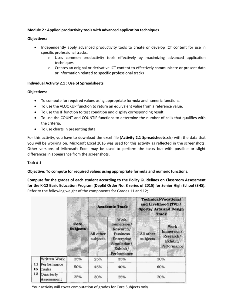
Compute for the grades of each student according to the Policy Guidelines on Classroom Assessment
for the K-12 Basic Education Program (DepEd Order No. 8 series of 2015) for Senior High School (SHS).
Refer to the following weight of the components for Grades 11 and 12;
Your activity will cover computation of grades for Core Subjects only.
These weights are also reflected on all 3 sheets of the excel file. Refer to the comments on respective
cells. Place mouse pointer on cell C4 on the Core Subject sheet, you should see the following:

You can view the other comments as well. You can add, edit or delete comments by clicking on
the Review tab for the options.
1.1 Compute for the Percentage Score for each of the component based from the Raw Scores
provided in the sheets.
Percentage Score (PS) is computed as;
PS = Total Raw Score / Highest possible score (HPS) * 100%
a. For the PS for written work, click on cell D5 and type the corresponding formula.
formula for D5
After pressing enter, you will see the results;
percentage
*You can also change the value to percentage by right-clicking the cell, choose format cell then
under category choose percentage.
b. To convert the result to percentage, click on the % symbol on the Home tab
percentage
c. For a more precise result, set the decimal places to two (2) by right-clicking on D5 and choosing
the option for Format Cells. Another window will launch, choose Percentage under category
and input 2 for Decimal places.
The value should be changed to 90.63%.
d. Compute for the PS of each of the remaining students. To do this quickly, you may just drag the
formula from D5 to D6 until D10. Click on D5, place mouse pointer on the lower right corner of
the cell where the mouse pointer changes to a black crosshair and drag down for all student
records. You will notice the following results;
What caused the problem? If you will click on any of the cell from D6 to D10, you will notice that the
formula changes, the value of C (C5/C16) is incrementing. Take for example D6, formula is
=(C6/C17)*100% , which should not be the case since the highest possible score(HPS) should not
change. Instead, the formula for D6 should be =(C6/C16)*100%. To ensure that C16 will not
increment you should place a $ sign before and after C in the formula for D5 from where you will
start dragging. This allows use of the absolute reference.
updated formula
Repeat the process for dragging the formula to compute for the PS of all students.
e. Repeat the process for computing the PS for Performance Tasks and Quarterly Assessment,
using corresponding raw scores and highest possible scores.
1.2 Compute for the Weighted Score for each of the component based from the Percentage Scores
computed.
Weighted Score (WS) is computed as;
WS = Percentage Score * Weight of Component
a. For the WS for written work, click on cell E5 and type the corresponding formula.
= D5 * E3
b. Format the result to 2 decimal places, this time under the category Number instead of
Percentage
c. Compute for the WS of the remaining students by dragging the formula. Make sure that the
value for weight component does not change and always refer to E3.
d. Repeat the process for computing the WS for Performance Tasks and Quarterly Assessment,
using corresponding percentage scores and weight components.
1.3 Compute for the Initial Grade of the students.
Initial Grade is computed as the sum of all WS from Written Work, Performance Task and Quarterly
Assessment.
Your output should look as follows;
Task # 2
Objective: To use the VLOOKUP function to return an equivalent value from a reference value.
Translate the Initial Grade to the Quarterly Grade and Descriptor using VLOOKUP.
*The VLOOKUP (Vertical lookup) function looks for a value in the leftmost column of a table, and then
returns a value in the same row from another column specified.
The transmutation table provided by DepEd will be used as reference;
*This is provided in the excel file as transmutation sheet.
2.1 Provide a name for the table that will be used to reference the equivalent transmuted value.
Highlight the cells that contain the values of the initial grade and the equivalent transmuted grade
(a2:a42,b2:b42) on the name box, type in transmutation as the name of the table.
name box
*Noticed that the values are arranged in ascending order and the value for initial grade does not use the
range but instead uses only the starting value in the range. When VLOOKUP looks for the transmuted
value, say for example 50, it looks at all values on the leftmost column (in this case column A) for the one
closest to 50 but not greater. The values closest but not higher than 50 is 48 which will then return the
value on the same row on the second column (in this case column B) which is 72.
2.2 Display the Quarterly Grade of all the students based from their initial grade.
The format for VLOOKUP function is
=vlookup(lookup value, table array, column index number, range lookup)
where : lookup value refers to the value you want to look up
table array refers to the range where you want to look up (either a range or name)
column index number refers to the column number in the range containing the return value
range lookup refers to the exact match or approximate match (usually same with lookup value)
a. Begin by providing the formula to provide the quarterly grade of the student Jose Burgos, click
on cell M5. Lookup value is the initial grade of Jose Burgos which is in cell L5; table array is
transmutation; column index number is 2 (column 2 in the table array where the quarterly
grade will come from); and range lookup is L5.
Formula should look like this :
= vlookup(L5, transmutation, 2, L5)
What will be the Quarterly Grade for Jose Burgos? Does it match with the values in the
transmutation table?
b. Do the same for all students. You can either provide the individual formula or just drag the
formula from M5. Don’t forget to counter check with the transmutation table.
2.3 Display the Descriptor of all the students based from their quarterly grade.
a. On the transmutation sheet, create a table array based from the following values and name it
descriptor.
*Follow the same principle applied for the transmutation table, make sure to arrange values in
ascending order and use only one value in the range. Remember that the grading scale refers to
the quarterly grade which will be the lookup value while descriptor will be the value displayed.
VLOOKUP function looks for a value in the leftmost column of a table
b. Provide the vlookup formula for all students. Don’t forget to check if the correct descriptor is
displayed for each student.
Task # 3
Objective: To use the IF function to test condition and display corresponding result.
Translate the quarterly grades to equivalent grade remarks using IF function.
*The IF function checks whether a condition is met, and returns one value if TRUE and another value if
FALSE.
3.1 Determine if the student PASSED or FAILED. A student passed if the quarterly grade is greater than
or equal to 75, and failed if quarterly grade is less than 75.
The format for the if function is:
= if(logical test, value if true, value if false)
Where:
Logical test refers to the condition being tested
Value if true refers to the displayed value once the logical test is true
Value if false refers to the displayed value once the logical test is false
*If function uses the logical operators = (equal), < (less than), > (greater than), <= (less than or
equal), >= (greater than or equal) and <> (not equal). Note that when the values to be tested or
displayed are strings (non-numeric values) they should be enclosed with a pair of quotations (“ “).
Start by determining the grade remark for Jose Burgos by using the if function. The logical test will
be to check if quarterly grade is greater than or equal to 75 to passed or if quarterly grade is less
than 75 which equates to failed. Either way, the correct results should be displayed.
Option 1:
= if (M5 >= 75, “Passed” , “Failed”)
Option 2:
= if (M5 < 75, “Failed”, “Passed”)
What grade remark was displayed for Jose Burgos using option 1 as formula? What about option 2?
Is the value displayed the same? Is it the correct remark?
3.2 Determine the grade remarks for the rest of the students.
Task # 4
Objective: To use the COUNT and COUNTIF functions to determine the number of cells that qualifies
with the criteria.
Display Grade Statistics using COUNT and COUNTIF functions.
*The COUNT function is used to count the number of cells that contain numbers. The COUNTIF function is
used to count the number of cells based on one criteria, while COUNTIFS is used to count the number of
cells based on multiple criteria.
The format for count function is:
=count (range of cells)
The format for countif function is:
=countif(range of cells, criteria)
The format for countif function is:
=countifs(range 1, criteria1, range 2, criteria 2, ….)
4.1 On the statistics sheet, provide the total number of students using count function. Use the
student quarterly grades from the core subject sheet for the range.
*To use the values from other sheets, you just need to click the corresponding sheet and click to the
specific cell or highlight a range of cells.
a.
To count total number of students, go to statistics sheet and click on cell C2, type in =count( to
choose the range go to core subject sheet highlight cell M5 o M14, your formula should look like
this; =COUNT('Core Subject'!M5:'Core Subject'!M14) and should display the value 10 on C2.
4.2 Count the number of students who passed and failed using countif.
a.
To count the number of students who passed, use the grade remarks from the core subject
sheet for the range and “passed” as the criteria. Your countif formula on cell C4 on the statistics
sheet should look like this; =COUNTIF('Core Subject'!O5:O14, "passed")
What was displayed? How many students passed? Is this correct?
b. Count the number of students who failed. Use appropriate formula to count failing students.
4.3 Using countif, determine the number of students whose descriptor is Outstanding, Very
Satisfactory, Satisfactory, Fairly Satisfactory and Did not meet expectations).
*Note that to match the criteria it has to be exactly the same in spelling and spacing. The criteria is
not case sensitive though.
Task #5
Objective: To use charts in presenting data.
Present the performance statistics in the core subjects using a chart.
*Charts are used to represent a sheet of numbers to a more visual and easy to compare statistics.
5.1 Using the data provided in the chart sheet, create a chart of the statistics of student grades in 4
core subjects.
a. Go to chart sheet, select the values that will be represented in the chart in this case A2:F6.
b. On the Insert tab, in the Charts group, choose Column or Bar chart
c. You will be provided with different column or bar chart formats, choose 2-D column. You will
notice that as you move the mouse pointer to different options the chart is also displayed.
d. Switch the row and column of the chart, go to Design tab and select Switch Row/Column
e. Add Chart Title and Axes Titles. Click on the label Chart Title to change title to Grade Statistics,
click on the plus (+) sign on the upper right corner of the chart to select Axis Title. Change axis
title to Number of Students and Subjects respectively.
*The Add Chart Element in the Chart Layouts group will also allow you to access Axis Title.
Your final chart should look like this.
*You can try other options for how you would want to display your chart. There are different types of
charts that are appropriate for specific presentations.