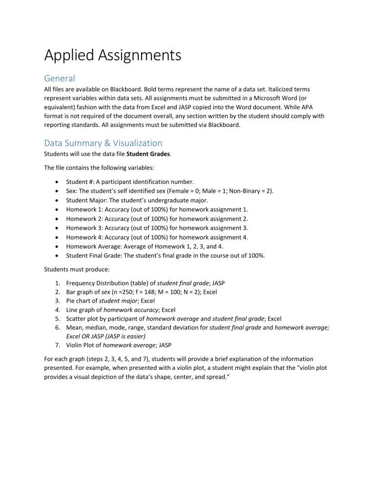
Applied Assignments
General
All files are available on Blackboard. Bold terms represent the name of a data set. Italicized terms
represent variables within data sets. All assignments must be submitted in a Microsoft Word (or
equivalent) fashion with the data from Excel and JASP copied into the Word document. While APA
format is not required of the document overall, any section written by the student should comply with
reporting standards. All assignments must be submitted via Blackboard.
Data Summary & Visualization
Students will use the data file Student Grades.
The file contains the following variables:









Student #: A participant identification number.
Sex: The student’s self identified sex (Female = 0; Male = 1; Non-Binary = 2).
Student Major: The student’s undergraduate major.
Homework 1: Accuracy (out of 100%) for homework assignment 1.
Homework 2: Accuracy (out of 100%) for homework assignment 2.
Homework 3: Accuracy (out of 100%) for homework assignment 3.
Homework 4: Accuracy (out of 100%) for homework assignment 4.
Homework Average: Average of Homework 1, 2, 3, and 4.
Student Final Grade: The student’s final grade in the course out of 100%.
Students must produce:
1.
2.
3.
4.
5.
6.
Frequency Distribution (table) of student final grade; JASP
Bar graph of sex (n =250; f = 148; M = 100; N = 2); Excel
Pie chart of student major; Excel
Line graph of homework accuracy; Excel
Scatter plot by participant of homework average and student final grade; Excel
Mean, median, mode, range, standard deviation for student final grade and homework average;
Excel OR JASP (JASP is easier)
7. Violin Plot of homework average; JASP
For each graph (steps 2, 3, 4, 5, and 7), students will provide a brief explanation of the information
presented. For example, when presented with a violin plot, a student might explain that the “violin plot
provides a visual depiction of the data’s shape, center, and spread.”
T-Test
Students will use a data file, Invisibility Cloaki. The file contains the following variables:



Participant: Identification number of a participant.
Cloak: Experimental group (0 = without a cloak of invisibility, 1 = with a cloak of invisibility).
Mischief: the number of mischievous acts committed by a participant.
We will test the hypothesis that students who use an invisibility cloak and those who do not use an
invisibility cloak engage in different amounts of mischievous acts.
Students must produce:
1. Independent Samples T-Test in which Mischief is the dependent variable and Cloak is the
independent variable (i.e., Grouping Variable, in this case). Students should select the correct
options to produce:
a. Location parameter (i.e., mean difference)
b. Effect Size (i.e., Cohen’s d)
c. Descriptives
d. Descriptive Plots with confident interval 95%
2. Brief writeup explaining the results of the t-test. The writeup should be 1 paragraph, include the
necessary statistics and their interpretation. An example is provided below:
One group of elementary students received a reading intervention, Directed Reading, and their reading
scores were compared to a control group at the end of the 8-week intervention. The treatment group
has on average about ten points more on the reading test than the control group, t(37.86) = 2.311, p =
0.013, which translates to a medium effect, Cohen’s d = 0.691ii,iii
One-Way ANOVA
Students will use a data file, Facebook Friendsiii,iv. The file contains the following variables:



Participant: Participant number.
Friends: Experimental group. The number of friends (the number indicates the number of
friended accounts with a mockup profile).
Score: Social attractiveness rating of the mockup profile (1 = lowest rating; 7 = highest rating).
We will test the hypothesis that as the number of friends increase, a profile’s social attractiveness score
increases.
Students must produce:
1. Descriptives by score and friends
a. Score is the variable of interest and should be moved to the variable box
b. Friends are our grouping variable; we’ll split by Friends.
c. Produce Boxplots with Boxplot and Violin elements.
2. ANOVA where in score is the dependent variable and friends is the independent variable
d. Under Additional Options, the student should check the Estimates of Effect Size box and
ensure that η2 is checked. Neither Partial η2 or ω2 should be checked.
e. Under Descriptive Plots, Friends should be moved to the horizontal axis. Display error
bars should be ticked.
3. Brief writeup explaining the results of the one-way ANOVA and the general trend of the
descriptive plot. The writeup should be 1 paragraph, include the necessary statistics and their
interpretation. An example is provided below:
The one-way ANOVA was significant, F(1,85) = 4.996, p = 0.028, η2 = 0.057, and suggest that it is unlikely
to observe these differences if the null hypothesis is true. The effect size indicates a modest effect and
suggests that 5 to 6 percent of the variance in social attractiveness ratings can be explained through the
number of friends an individual has on their social media page.
Single-Case Design
COMING SOON TO AN ASSIGNMENT SHEET NEAR YOU.
Regression
Students will use the data file Student Grades.
Recall that we used this data set in the first activity (see page 1 for details). We have already produced
descriptives of these data and visualized key aspects. We want to know if Homework average can
predict Student Final Grade.
Students will produce:
1. Correlation plot of Homework Average and Student Final Grade.
2. Linear Regression predicting Student Final Grade with Homework Average.
4. Students will produce 1-2 sentences explaining the findings of the simple linear regression (with
focus on R2) and the coefficients table (with focus on t and p). An example is provided below:
Example:
Model Summary
1
Coefficients
R
0.578
Variable
Average Homework
R2
0.335
Unstandardized (SE)
.86 (.010)
F(df) p
99.59(1,198), <.001
T (p)
19.979(198), < .001
Note. Some elements have been combined from JASP output. Other elements (e.g., standardized estimate) have been
eliminated. These steps were taken for clarity. These data are simulated and should not be used for your assignment. These
data would be found in the Model Summary (i.e., R, R2), ANOVA (i.e., F, df, and p), and Coefficients (i.e., unstandardized
estimate, standard error [SE], t, df, and p values) tables.
The model suggests that Average Homework predicts Student Final Grade fairly well, as it explains 33.5%
(R2 = 0.335) of the variance in the final grade. Additionally, observing this pattern (or a more extreme
one) is highly unlikely if Homework Average and Student Final Grades were not related to each other,
F(1,198) = 99.59, p < .001. Finally, as a student’s Average Homework grade increases by 1 point, the
Student’s Final Grade increases by .86 (unstandardized = .86, t(198) = 19.979, p > .001) points.
i
Field, A. P. (2017). Discovering Statistics Using IBM SPSS Statistics (5th ed.). London: Sage. [Fictional data set].
ii
Schmitt, M. C. (1978). The effects of an elaborated directed reading activity on the metacomprehension skills of
third graders. PhD thesis, Purdue University.
iii
iv
D. S. Moore, G. P. McCabe, & B. A. Craig. Introduction to the practice of Statistics (7 th ed.). New York: Freeman.
Tong, S. T., Van Der Heide, B., Langwell, L., & Walther, J. B. (2008). Too much of a good thing? The relationship
between number of friends and interpersonal impressions on Facebook. Journal of Computer-Mediated
Communication, 13.