Color Interpolation for Cross-Talk Noise Reduction
Wen-Han Chen(陳文漢), Chiou-Shann Fuh(傅楸善)
Graduate Institude of Networking and Multimedia, National Taiwan University, Taipei, Taiwan
Abstract—Most digital cameras use single electronic sensors
colors of light. When the digital camera sensor catches the
such
CMOS
light, the color filter array will absorb the light based on
(Complementary Metal-Oxide-Semiconductor). To reduce cost,
different wavelengths of light. Furthermore, to transform the
we always use Bayer pattern to get the other color information.
photon to electron signal, we get raw image, the original data
Since white light is composed of light of different wavelengths.
which sensor captures. If we want to get the other color
Since silicon has different absorption rates for different
channel
wavelengths. It will cause blocky cross-talk artifact. In this
interpolation algorithm to get the other color information.
as
CCD
(Charge-Coupled
Device)
or
thesis, we propose a new color interpolation to reduce blocky
information and successfully keep image detail.
value
for
corresponding
pixel,
use
color
Initially, there are many types to arrange color pixel
photosensor. But now most popular on consumer digital
camera is Bayer filter. In 1976 Bryce Bayer’s patent [1], he
Keywords- color interpolation, cross-talk noise, false color
1.
INTRODUCTION
uses retina characteristic where rod cells are more sensitive
to green light and human eye are sensitive to three primary
Digital camera usually uses Color Filter Array (CFA) to
color light. Therefore, he uses 50% green, 25% red, and 25%
capture scene color value. Using color filter array reduces
blue elements. The final image result is called Bayer pattern
cost. Because of color array, we face a special image
image.
structure, Bayer pattern [1]. Raw image contains mosaic data.
Similarly, the other alternative filter on digital camera, such
Each pixel only has one color channel value, such as Green
as RGBE (Red, Green, Blue, and Emerald) used in Sony
pixel between two Red pixels in the same row. If we want to
digital camera serious, CYGM (Cyan, Yellow, Green,
get a complete color and good quality image, demosaicking
Magenta) uses alternative pattern to record three primary
Bayer pattern value is necessary, also called color
colors.
interpolation. A good color interpolation algorithm can
1.2 Pixel Cross-Talk
reduce false color and keep the detail successfully. In this
thesis, we present a new color interpolation algorithm and it
can remove common artifact, such as cross-talk which
creates blocky noise or image edge zipper effect and blurred
edge.
1.1 Color Filter Array
To reduce cost, Color Filter Array (CFA) arranges red,
green, and blue pixel sensor as in Figure 1.1 instead of using
three sensors at the same location to catch three primary
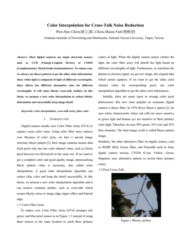
Figure 1 Blocky artifact.
For Charge-Coupled Device (CCD) or Complementary
original Bayer pattern value to compute image
Metal-Oxide Semiconductor (CMOS) image sensor to
gradient. Edge pixel has higher continuity than the
capture scene value, cross-talk usually occurs. Neighbors
other. Thus we interpolate blank pixel based on
may interfere with central pixel value. Many possible
gradient.
reasons, such as incident light angle may cause adjacent
2.2 Cross-Talk Compensation Method
sensor to absorb redundant photons to convert into electronic
Generally, there are two algorithms to compensate cross-
signal. Moreover, silicon absorption ratios for light of
talk [7]. Because human eyes are sensitive to green color, in
different wavelengths are different. Horizontal and vertical
Bayer pattern, we adjust Gr and Gb channel values. We
adjacent pixels have different influences on neighbor pixels.
estimate the gradient and local average to keep image
Due to pixel layout direction, the horizontal neighbors have
sharpness and reduce cross-talk phenomenon.
higher influence than vertical neighbors. Result image at the
2.2.1 Interpolation-Based Method
smooth region usually has blocky zigzag.
2.
RELATED WORK
2.1 Color Interpolation Method
2.1.1 Nearest-Neighbor Interpolation
Nearest neighbor is the simplest color
interpolation algorithm. Its concept is rounding-off
error to get an approximation to get the nearestneighbor integer value. Advantages are simple, easy,
and fast implementation. On the other hand,
Figure 2 Interpolaton-based method [7]. (a) Bayer pattern
has four possible arrangements, i.e. first column: one red
value between Gr channel. (b) First column: one blue value
between Gb channel.
disadvantages are zigzag between neighbors and
obvious line artifact between each pixel.
2.1.2 Bilinear Interpolation
In one dimension, we usually use linear
In [7], based on an assumption, we try to equalize Gr
and Gb channels. In Figure 2.4.a, if we use Gb as a reference
channel, we want to get Gr at G7 location. We can assume
that
interpolation to get an unknown value. Most digital
G7new  G7  G7
image use F(x): Z2 → N3 to describe one position
with three integer color channel values. Thus at two
dimensions, we use linear interpolation twice on
horizontal and vertical directions.
2.1.3 Edge-Sensing Interpolation
Where
G4
Most common color interpolation algorithm has
the same problems which produce false color on edge
region. In human visual system, most people are
sensitive at edge pixel and luminance change.
According to the characteristic, we refer to the
(G4  G5  G9  Ga )
4
(G  G2  G6  G7 )
 G4  1
4
(G  G3  G7  G8 )
 G5  2
4
(G  G7  Gb  Gc )
 G9  6
4
(G7  G8  Gc  Gd )
 Ga 
4
G7 
G5
G9
Ga
Or we can simplfy equations
G7new 
G4  G5  G9  Ga 12G7  [2(G2  G6  G8  Gc )  G1  G3  Gb  Gd ]

4
16
where X(p,q)1 means Red color value; X(p,q)2 means Green
value; and X(p,q)3 means blue value. We post-process to
reduce false color in final image [9]. Color interpolation aims
choose Gr (Figure 2.4.b) or Gb as a reference channel, the
to use original raw data for final color correction.
most important thing is to keep the two channels equalized.
At Section 2.3, color correlates significantly in a small
2.2.2 Average-Based Method
In [7], the other method to remove cross-talk exists. Use
region. After getting the final image, we use three channels
to correct color value for each position.
a local average to keep green channel balanced, without
adjusting one of them. In Figure 8.a we can derive formula
G7  (Gr  Gb )
2
G4  G5  G9  Ga
Gr 
4
G1  G2  G3  G6  G7  G8  Gb  Gc  Gd
Gb 
9
G7new 
These algorithms can be implemented as an independent
function before color interpolation. It helps for pipeline
function implementation and performance improvement.
2.3 Color Difference Planes
In [8], for Bayer pattern, each position only has one
channel value. But image has high correlation between each
channel in a small region. We can use the characteristic to
develop image model.
Kr  G  R
Kb  G  B
Figure 3 (a) First, fill green value with dimond mask. (b)
Second, fill each blank blue or red central value with square
mask. (c) and (d) Fill the other blank pixels [9].
In Figure 3(a) we select the original green value position
at the corresponding raw data. Then use the following
formula.
X  p ,q 2  X  p ,q k  ?

( i , j )
w(i , j ) ( x(i , j )2  x(i , j ) k )
green value subtracted by blue value. Use the new color
domains Kr and Kb to interpolate red and blue planes. By
transformation, we interpolate green channel and KrKb
channel. Finally, we similarly interpolate blue and red
channels. In Figure 10 we can find out it is smoother in hue
domain. This is good for interpolation and reduces false

( i , j )
Kr means green value subtracted by red value, and Kb means
w(i , j )
Moreover, weighting coefficient calculation is
w(i, j ) 
d (i, j ) 
1
1  d (i, j )

( g , h )
x(i , j )2  x( g ,h )2
where   {( p  1, q), ( p, q 1), ( p, q  1), ( p  1, q)}
color.
2.4 False Color Removal
In a full color image, we use a vector X(p,q) = (X(p,q)1,
X(p,q)2, X(p,q)3) ∈ Z2 to describe three color components
Choose a diamond mask to select neighbors and adjust
green value by color correlation.
Second, we find the red/blue corresponding position at
original raw data. Select a square mask and fill central pixel
value as follows.
3.
OUR PROPOSED METHOD
In this chapter, we will present my method. First, we
separate raw data in three planes: red, green, and blue planes.
X(p,q)k = X(p,q)2 +
 w
(i , j )
( i , j )
( x(i , j ) k  x(i , j )2 )

( i , j )
To reduce cross-talk noise in raw data, we use a reference
channel such as Gr or Gb. Then adjust each green channel
w(i , j )
value according to local average value. Then, we use blue
and red information to build color correlation planes Kr and
where 
 {( p  1, q  1), ( p 1, q  1), ( p  1, q 1), ( p  1, q  1)}
Kb to avoid false color, but Kr and Kb have many blank
After second step, we use the previous diamond to fill
positions. Thus we use linear interpolation twice to fill these
red/blue plane and get the final image. It is good to
blank pixels. Finally we inverse Kr and Kb planes to
implement pipeline and improve performance after we get
corresponding red and blue values and use a false color
the final image.
removal function to correct final image. this property, we
2.4 Edge Sensing Mechanism
can set a mask with border, if we find many edge pixels
In Section 2.4, the weighting calculation uses edge
around middle pixel, but we can not find any edge pixel in
sensing mechanism. We calculate gradient to decide
the border of mask. By this judgment, this mask presumes it
weighting coefficient. If we get a great gradient value, it
is a noise cluster, and eliminates it. In H.Y. Shen’s method
means that there is an edge across the small region. On the
[5], this function can be canceled if we want to keep more
other hand, small gradient value means that mask covers a
detail. Usually, the mask size is 5*5~15*15 pixels.
smooth region.
3.1 Calculate Gradient Difference
d (i, j ) 

( g , h )
x(i , j ) k  x( g ,h ) k
With large gradient magnitude, we need to reduce
neighbor effect for central pixel. Practically, we usually use a
simple function as follows
w(i, j ) 
1
1  d (i, j )
Use inverse function to control coefficient effect.
Moreover, denominator always adds one to avoid d(i,j) to be
too small.
Figure 5 Calculate four directions.
In real world, raw data usually have cross-talk noise.
The artifact always rises at smooth region. We want to
separate image region into smooth and non-smooth regions.
Figure 4 (a) Square lattice. (b) Quincunx lattice [10].
In this step, we calculate gradient in four directions. In
Kr3 
Figure 3.1.2, interesting pixel is G13.
H  G11  G15
Kr 7 
V  G3  G23
Kr9 
C1  G7  G19
K r13 
C2  G9  G17
 Kr 2 
Kr 4 
2
K

 r 2 K r12 
2
 K r 4  K r14 
2
 K r12  K r14 
2
Symbol H means horizontal direction; V means vertical
Final remaining blank position will be near four Kr/Kb
direction; C1 and C2 mean two diagonal directions. If the
pixels. We use bilinear interpolation to fill these blank
5X5 mask covers a smooth region, these gradient
differences will be small. We use the information to avoid
false color with green channel compensation.
pixels.
Kr8 
 Kr 3 
K r 7  K r 9  K r13 
4
3.3 Re-Interpolate G, Kr, and Kb
( H  V  C1  C2 )
 Threshold
4
 edge cross 5  5 mask
If
In Section 3.2, we set Kr/Kb by reference green channel
value at corresponding position. To promote precision, we
recalculate three channel values.
else
 smooth region
3.2 Set Kr and Kb Planes and Interpolate
In this step we use original red and blue data to subtract
corresponding green plane value. In Figure3.1.2, we want to
set Kr plane first.
K r 2  G2  R2
K r 4  G4  R4
K r12  G12  R12
K r14  G14  R14
Previously, we have gotten an entire green channel
Figure 6 Original raw data format.
plane to use this information to estimate Kr and Kb planes.
Thus we will get Kr and Kb planes. There are many blank
First we re-interpolate green channel plane. In Figure 3.1.3,
positions. We fill horizontal and vertical blank positions by
we can find out B7 has no green value in original data.
linear interpolation between two Kr/Kb pixels.
K b 6  G6  B6
K b8  G8  B8
K b 2  G2  B2
K b12  G12  B12
Then we can use original blue value B7 to estimate G7 as
follows
G7  B7 
 Kb6  Kb8  Kb 2  Kb12 
4
The red position is the same.
Second, we want to re-interpolate Kr and Kb planes. To
estimate Kr and Kb, we estimate G minus original R/B to set
up corresponding planes. Now we have three color planes to
rebuild it. In Figure2.1.3 we can reset Kr as follows
Original Image1
Raw data: 10 bits/pixel
Image size: 2592*1944 pixels
Bayer pattern: BGbGrR
K r 3  G3  R3
K r 7  G7  R7
K r 9  G9  R9
K r13  G13  R13
Similarly for Kb. In the new Kr and Kb, we can use bilinear
interpolation to interpolate blank position.
Kr8 
4.
 Kr 3 
K r 7  K r 9  K r13 
4
EXPERIMENTS AND RESULTS
Experimental Environment
CPU: AMD Athlontm II X2 245 Processor 2.90 GHz
Memory: 4 GB
OS: Windows 7 Professional
Programming Language: Microsoft Visual Studio 2008
with OpenCV 2.0
Bilinear: 0 votes
CDb: 2 votes
Our Method: 19 votes
(CD: Color Difference with bilinear interpolation)
Original Image2
Raw data: 10 bits/pixel
Image size: 2592*1944 pixels
Bayer pattern: BGbGrR
Our Method: 20 votes CDb: 0 votes
Original Image3
Raw data: 10 bits/pixel
Image size: 2592*1944 pixels
Bayer pattern: BGbGrR
Bilinear: 1 votes
CDb: 4 votes
5.
Our Method: 17 votes Bilinear: 0 votes
CONCLUSION AND FUTURE WORK
5.1 Conclusion
Traditional color interpolation uses Kodak sample images to
calculate PSNR (Peak Signal-to-Noise Ratio). Our method
designs for real raw data but Kodak sample image has no
common artifact, such as false color and cross-talk noise.
Thus, we use real raw data and votes to show our method
results. In real raw data, our method reduces cross-talk noise
for Demosaicking: A Framework,” IEEE Transactions on
and false color successfully. But bad pixel or fixed pattern
Consumer Electronics, Vol. 51, No. 2, pp. 560-570, 2005.
noise affect our method to determine which region is
[8]
S. C. Pei, I. K. Tam., “Effective Color Interpolation in
smooth or not. Noise has outlier pixel characteristic. In
CCD Color Filter Arrays Using Signal Correlation,” IEEE
gradient calculation, we may determine it as an edge across
Transactions on Consumer Electronics, Vol. 13, No. 6, pp. 503-
this mask. If we can reduce noise effect, image after color
513, 2003.
interpolation will get higher quality than before.
[9]
5.2 Future Work
can develop a function to determine whether each pixel in
the mask is outlier pixel or not, it will be useful for our
method to determine whether central pixel needs
compensation or not. Thus we can further enhance image
quality.
REFERENCES
B. E. Bayer, “Color Imaging Array,” US Patent
#3971065, 1976.
[2]
T.
Chen,
“Bilinear
Interpolation,”
http://scien.stanford.edu/pages/labsite/1999/psych221/projects/99/
tingchen/algodep/bilinear.html, 2011.
[3]
T. Chen, “Edge Sensing Interpolation Algorithm I,”
http://scien.stanford.edu/pages/labsite/1999/psych221/projects/99/
tingchen/algodep/edgesense.html, 2011.
[4]
T.
Chen,
“Nearest
Neighbor
Replication,”
http://scien.stanford.edu/pages/labsite/1999/psych221/projects/99/
tingchen/algodep/nbreplica.html, 2011.
[5]
W. Li, P. Ogunbona, Y. Shi, and I. Kharitonenko,
“CMOS Sensor Cross-Talk Compensation for Digital Cameras,”
IEEE Transactions on Consumer Electronics, Vol. 48, No. 2, pp.
292-297, 2002.
[6]
R. Lukac and K. N. Plataniotis, “A Robust, Cost-
Effective Post-Processor for Enhancing Demosaicked Camera
Images,” Journal of Real-Time Imaging, Vol. 11, Issue 2,
pp.139–150, 2005.
[7]
“Bayer
Filter,”
http://en.wikipedia.org/wiki/Bayer_filter, 2011.
In Section 3.1, we determine pixel is an edge or not. If we
[1]
Wikipedia,
R. Lukac and K. N. Plataniotis, “Data Adaptive Filters
[10]
Wikipedia,
“Color
Filter
http://en.wikipedia.org/wiki/Bayer_filter, 2011.
Array,”