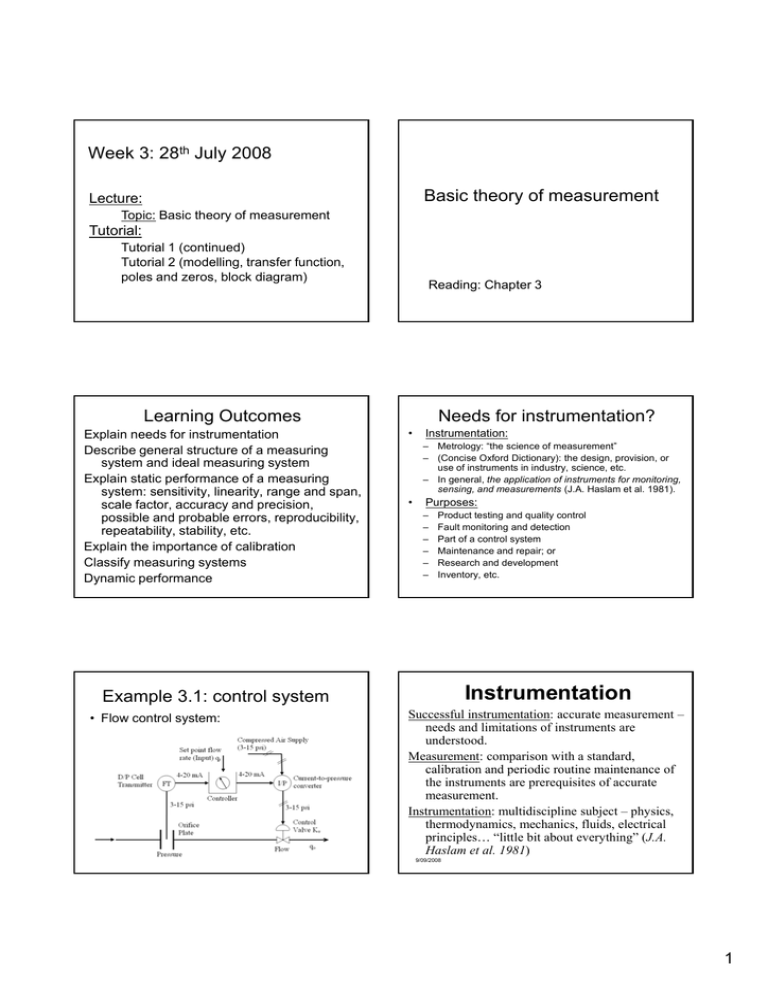
Week 3: 28th July 2008
Basic theory of measurement
Lecture:
Topic:
p Basic theoryy of measurement
Tutorial:
Tutorial 1 (continued)
Tutorial 2 (modelling, transfer function,
poles and zeros, block diagram)
Reading: Chapter 3
Learning Outcomes
Explain needs for instrumentation
Describe general structure of a measuring
system and ideal measuring system
Explain static performance of a measuring
system:
y
sensitivity,
y, linearity,
y, range
g and span,
p ,
scale factor, accuracy and precision,
possible and probable errors, reproducibility,
repeatability, stability, etc.
Explain the importance of calibration
Classify measuring systems
Dynamic performance
Needs for instrumentation?
•
Instrumentation:
– Metrology: “the science of measurement”
– (Concise Oxford Dictionary): the design, provision, or
use of instruments in industry, science, etc.
– In general, the application of instruments for monitoring,
sensing, and measurements (J.A. Haslam et al. 1981).
•
Purposes:
–
–
–
–
–
–
Product testing and quality control
Fault monitoring and detection
Part of a control system
Maintenance and repair; or
Research and development
Inventory, etc.
Instrumentation
Example 3.1: control system
• Flow control system:
Successful instrumentation: accurate measurement –
needs and limitations of instruments are
understood.
Measurement: comparison with a standard,
calibration and periodic routine maintenance of
the instruments are prerequisites of accurate
measurement.
Instrumentation: multidiscipline subject – physics,
thermodynamics, mechanics, fluids, electrical
principles… “little bit about everything” (J.A.
Haslam et al. 1981)
9/09/2008
1
General Structure of
Measuring System
Transduced
signal
Primary
qquantityy
Transducer
Physical
variable
Measurand
Sensor
Converter
Transmitter
Measuring system
Conditioned
signal
Signal
Conditioner
Recorder or
Indicator
Converter
Amplifier
Display
Pen recorder
Printer, etc.
9/09/2008
Simple measuring system
Complicated measuring system with amplifier,
A/D converter, and computer output
System Performance
• Ideal measuring system: where the output signal has
a linear relationship with the measurand (quantity to
be measured), where no errors are introduced by
effects such as static friction, and where the output
is a faithful reproduction of the input no matter how
the input
p varies.
• Static Performance: when steady or constant input
signals are applied, comparison of the steady output
with the ideal case gives the static performance of
the system.
• Dynamic Performance: when changing input signals
are applied, comparison with the ideal case gives
the dynamic performance of the measuring system.
Static Sensitivity
• Static sensitivity is the ratio of the change
in output to the corresponding change in
input under static or steady state
conditions.
K=
Δy
Δu
Δy
Δu
the change in output
the change in input
Unit depends on the instrument or measuring
system being considered.
Static Performance
•
•
•
•
•
•
Sensitivity
Range, Span
Accuracy and Precision
Linearity
Possible and Probable Errors
Other Static Performance Terms:
Reproducibility, Repeatability, Stability,
Constancy, Tolerance, Resolution,
Dead-band, Hysteresis.
Sensitivity: Example 3.2
A measuring system: a transducer, an
amplifier, and a recorder:
K1 = 0.2 mV/oC
Transducer (oC-mV):
Amplifier (mV-V):
K2 = 2.0 V/mV
Recorder (V-mm):
K3 = 5.0 mm/V
K = K1 × K 2 × K 3
K = 0.2( mV / o C) × 2.0( V / mV ) × 5.0(mm / V )
K = 2.0mm / O C
2
Example
A temperature-measuring system incorporates
a platinum resistance thermometer, a
Wheatstone bridge, a voltage amplifier, and
a pen recorder. The individual sensitivities
are transducer: 0.35 ohm/oC, Wheatstone
bridge: 0.01 V/ohm, amplifier gain: 100 V/V,
and pen recorder: 0.1 cm/V
Determine:
1. the overall system sensitivity
2. temperature change corresponding to a
recorder pen movement of 4 cm
Linearity
The ratio of the maximum deviation from a linear
relationship (ideal) between the input and output to the
maximum scale – expressed as percentage of full scale.
Vmax
Indicated (V)
ΔV
ΔV
Linearity(%) =
×100%
Vmax
Actual (V)
Example 3.3: Linearity
An ohmmeter used to measure
resistance in range of 0 to 200 Ohms
gave the maximum deviation of 2.0
Ohms. The linearity is as follows
Linearity(%) =
2.0V
×100% = 1.0(%)
(200 − 0)Ω
Range, Span
Range of a variable is a numerical statement
of the minimum and maximum values that
the variable can assume. A DC voltmeter:
0V-30V, mA-meter: 4mA-20mA
p is the numerical difference between two
Span
range values. DC voltmeter: 30V-0V = 30V,
mA-meter: 20mA-4mA = 16mA
Scale Factor is a number which scales or
multiplies the physical quantity to be
measured: SF=Sy/Sx or Sy=SF*Sx
More example
• Data from a dc tachometer test:
• Determine the linearity in the full scale?
– Least squares to find ideal relationship
– Calculate the maximum deviation
– Calculate the linearity.
Accuracy and Precision
• Accuracy is normally stated in terms of
errors introduced, where
indicated value − true value
× 100%
true value
The error as a percentage of the measuring
range of the equipment:
error (%) =
error (%) =
indicated value − true value
× 100%
max scale value
3
Accuracy and Precision
• Precision does not mean accuracy. An instrument
provides reading which are very close in value it is
said to have high precision.
• Ap
precise measurement may
y not be an accurate
measurement.
• When repeating measurements of the same input
for several times the indicated readings lie closely
together, the instrument is said to be of high
precision. The accuracy means the closeness of
the indicated readings to the true values.
Examples of Error
A 0-10bar pressure gauge: error of +/0.15bars when calibrated by manufacturer.
(a) Percentage error of the gauge:
0.15bars
× 100% = ±1.5%
10bars
(b) Possible error when reading of 2.0bars:
E
Error
(%) =
Error (%) at 2.0bars =
0.15bars
× 100% = 7.5%
2.0bars
Sources of Error
Incorrect observation, incorrect position or graduation
of scale… significant sources of error which combine
to affect adversely the accuracy of measurements:
z Friction, backlash, & inertia (mechanic)
z Hydraulic friction, leakage, & inertia (hydraulic)
z Heat loss through imperfect insulation and imperfect
thermal conductivity
z Distributed pneumatic capacitance & resistance
z Offset, drift, effects of distributed resistance,
conductance, & capacitance, etc.
Illustration of difference between
accuracy and precision
True value
H.A.
H.P.
L.A.
H.P.
L.A.
L.P.
Example
A 0-100oC thermometer is found to
have a constant error of +0.2oC.
Calculate the percentage error at
readings of
(a) 10oC,
(b) 50oC and
(c) 100oC
Possible and Probable Errors
Maximum possible error:
Maximum possible error =
± (a + b + c)%
Probable error:
Root-sum-square error =
± a 2 + b 2 + c 2 (%)
Example: ± 2% ± 3% ± 5%
Effect of disturbance and noise in Ch 16
4
Other static-performance terms
• Reproducibility: A general term applied to the
ability of a measuring system or instrument
to display the same reading for a given input
applied on a number of occasion.
• Repeatability: The reproducibility when a
constant input is applied repeatedly at short
intervals of time under fixed conditions of use.
• Stability: The reproducibility when a constant
input is applied over long periods of time
compared with the time of taking a reading,
under fixed conditions of use.
Standards and Calibration
Standards:
z Requirement for more accurate measurements has evolved as
human beings have developed more complex and sophisticated
technologies.
z Standards help to make devices manufactured in different
places compatible to each other.
z It is important to understand the need for calibration and
adjustment
dj t
t off test
t t and
d production
d ti equipment.
i
t
z Australian Standards Organization in Sydney, NSW.
Calibration:
z Calibration is the process of adjusting test and production
equipment to conform to standards, and verifying (certifying)
their compliance to those standards.
z Calibration methods and period are often instructed by
manufacturer of the equipment.
Dynamic Performance
• The dynamic performance of both measuring and control
systems is extremely important and is specified by
responses to certain standard test inputs.
• Step input: which takes the form of an abrupt change from
one steady value to another. This indicates how well the
system can scope with the change and results in the
transient response.
response
• Ramp input: which varies linearly with time and gives the
ramp response, indicating the steady-state error in following
the input.
• Sine-wave input: which gives the frequency response or
harmonic response of the system. This shows how the
system can respond to inputs of a cyclic nature as the
frequency f (Hz) or ω (rad/s, ω=2πf) varies.
Other static-performance terms
• Tolerance: The maximum error.
• Resolution: The smallest change of input to an instrument
which can be detected with certainty, expressed as a
percentage of full scale.
• Dead-band: The largest change of input to which the system
does not respond due to friction or backlash effects,
expressed as a percentage of full scale.
• Hysteresis: The maximum difference between readings for
the same input when approached from opposite directions,
I.e. when increasing and decreasing the input, expressed as
a percentage of full scale.
• Constancy: The reproducibility when a constant input is
presented continuously and the conditions of test are
allowed to vary within specified limits, due to some external
effect such as a temperature variation.
Classification of MSs
Types of signal: analogue, digital and hybrid
(combination of analogue and digital)
Types of physical processes: mechanical,
hydraulic, pneumatic, electrical and
electronic (microprocessor/computer based)
Trend shows an increase of electronic and
computer-based measuring equipment
because of rapid speed of response, ease
with electrical signals, digital and graphical
visualization, and reliability and
programmability
Dynamic Performance
• All systems will to some extent fail to follow
exactly a changing input; and a measure of
how well a system will respond is indicated
by its dynamic specifications (step or
transient parameters or frequency-response
frequency response
parameters)
• Many systems, although different in nature,
produce identical forms of response – the
system dynamics are similar
5
Test Input Signals
It is necessary for the designer to test
the performance of a measuring or
control system using test input signals.
Test Inputs: Typical test inputs: step,
ramp and sine wave
Step
Ramp
Zero-Order System
• Zero-order measuring system
y = Ku
• Step input – step response
• Ramp input – ramp response
• Sine wave input – frequency response
Sine wave
9/09/2008
Examples of zero-order
measuring systems
• Potentiometer (output voltage proportional to
the displacement of the wiper)
• The zero-order
zero order measuring system has an
important property: that the output is
proportional to the input no matter how the
input varies – ideal measuring system.
First-order Systems
• First-order measuring system (standard
form)
τ
τ
dy
+ y = Ku
dt
H=
K
τs + 1
time constant
K: static sensitivity
• Step input, ramp input and sine wave input
Examples of first-order
measuring systems
• Mercury-in-glass thermometer, build-up
pressure in a resistor/bellows
of air p
system, a series resistance-capacitance
network, etc.
Example
• Mercury-in-glass thermometer, where
the heat conduction through the glass
bulb to the mercury is described by a
first-order differential equation:
dy
+ 2 y = 2 × 10 −3 u
dt
dy
T = 2sec
2 + y = 10 −3 u K = 10-3m/oC
dt
4
6
Example
Second-order System
Determine the time constant and the static sensitivity
of the systems
dy
a)
30 + 3y = 1.5 ×10 −5 u
• Second order measuring system
d2 y
dy
+ 2ξωn
+ ω2n y = ku
dt 2
dt
y(s)
K
=
u (s) (1 / ω2n )s 2 + (2ξ / ωn )s + 1
dt
for a thermocouple in a protective sheath
sheath, where y =
output voltage in V and u = input temperature in oC.
dy
b)
1.4
dt
+ 4.2 y = 9.6u
for a resistor/bellows system, y = bellows
displacement in mm, and u = input pressure in bars
ξ
is a measure of the damping present in a system and is
equal to the ratio of actual damping to critical damping
a measure of the speed of response of the secondωn isorder
system – higher values of ω would mean that the
n
system would response more rapidly to sudden changes
Second-order System
Example of 2nd-order system
• The dynamic performance of a piezo-electric
accelerometer can described by the following
differential equation:
d2y
dy
+ 3.0 × 103
+ 2.25 ×1010 y = 11.0 × 1010 u
2
dt
dt
where y = output charge in pC, and u = input
acceleration m/s2.
By comparison with the standard equation,
determine the values of ωn, ξ and the static
sensitivity K.
(ans: 1.5*105, 0.01, 4.89pC/(m/s2))
Examples of second-order
measuring/control system
ξ < 1: The system is said to be underdamped and results
in oscillations occurring in the step response and (for
values of ξ < 0.707) resonance effects in the
frequency response.
ξ = 1: This is the critically damped condition: ie no
oscillations or overshoots appear in the step response
and there is no resonance in the frequency response.
This is the point of change-over from an underdamped
condition to an overdamped condition.
ξ > 1: The system is overdamped in the step response
and no resonance in the frequency response.
Example: Step-response Specs
140
120
• Mass-spring system with damping, yaw
angle vs rudder system (Nomoto). A
l
large
number
b off d
devices
i
and
d
mechanisms.
• Simulation in MATLAB/Simulink
(illustrates responses with different values
of ξ and ωn)
100
80
d2y
dy
+ 2 × 1 × 0 .4 + y = u
2
dt
dt
60
40
20
0
0
1
2
3
4
5
6
7
8
9
10
Effect of disturbance and noise in Ch 16
7
Summary
• Definition and concepts of instrumentation, needs
for instrumentation, ideal measuring system,
structure of a measuring system
• Static performance of a measuring system:
sensitivity, range, span, scale factor, accuracy and
precision,
i i
lilinearity,
it possible
ibl and
d probable
b bl errors,
reproducibility, repeatability, stability, constancy,
tolerance, resolution, dead-band, hysteresis.
• Standards & calibration
• Classification of measuring systems
• Dynamic Performance: test input signals
Any questions?
Tutorials
• Solving differential equations using
Laplace transform
• Modelling: derive differential equations
• Transfer
T
f function
f
ti
• Poles and zeros
• Block diagram
8