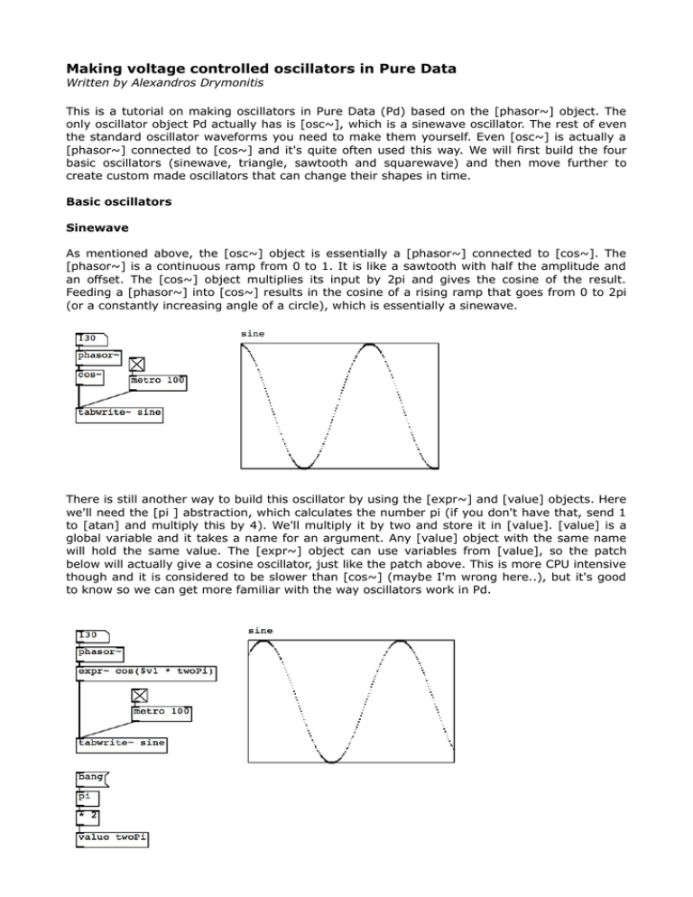
Making voltage controlled oscillators in Pure Data
Written by Alexandros Drymonitis
This is a tutorial on making oscillators in Pure Data (Pd) based on the [phasor~] object. The
only oscillator object Pd actually has is [osc~], which is a sinewave oscillator. The rest of even
the standard oscillator waveforms you need to make them yourself. Even [osc~] is actually a
[phasor~] connected to [cos~] and it's quite often used this way. We will first build the four
basic oscillators (sinewave, triangle, sawtooth and squarewave) and then move further to
create custom made oscillators that can change their shapes in time.
Basic oscillators
Sinewave
As mentioned above, the [osc~] object is essentially a [phasor~] connected to [cos~]. The
[phasor~] is a continuous ramp from 0 to 1. It is like a sawtooth with half the amplitude and
an offset. The [cos~] object multiplies its input by 2pi and gives the cosine of the result.
Feeding a [phasor~] into [cos~] results in the cosine of a rising ramp that goes from 0 to 2pi
(or a constantly increasing angle of a circle), which is essentially a sinewave.
There is still another way to build this oscillator by using the [expr~] and [value] objects. Here
we'll need the [pi ] abstraction, which calculates the number pi (if you don't have that, send 1
to [atan] and multiply this by 4). We'll multiply it by two and store it in [value]. [value] is a
global variable and it takes a name for an argument. Any [value] object with the same name
will hold the same value. The [expr~] object can use variables from [value], so the patch
below will actually give a cosine oscillator, just like the patch above. This is more CPU intensive
though and it is considered to be slower than [cos~] (maybe I'm wrong here..), but it's good
to know so we can get more familiar with the way oscillators work in Pd.
Triangle
The triangle oscillator is, out of the standard oscillators, the most complex to build. We're
based on [phasor~] which is an upward ramp from 0 to 1. In order to get a triangle out of this
shape we'll need to do some tweaking. First we'll need a copy of [phasor~] with an inverted
direction. To get this, we'll need to multiply [phasor~] by -1, so now the ramp will go from 0 to
-1. Then we'll need to add 1, so now the ramp goes from 1 to 0.
We now have the copy with the inverted direction. If we send both the [phasor~] and its
inverted copy to [min~], we obtain a triangle that goes from 0 to 0.5. [min~] will take two
input values and output the smallest one. Sending it a rising and a falling ramp, for half the
period it will output the rising ramp (at the beginning [phasor~] is at 0 and the inverted copy
at 1), and for the other half the falling one. As they both meet at 0.5, our triangle will have a
span of 0.5.
Since oscillator waveforms have a span of 2 (from -1 to 1) we'll need to multiply our triangle
by 4 and we'll get a new triangle that goes from 0 to 2. Finally subtracting 1 will offset our
triangle from -1 to 1.
Sawthooth
The sawtooth waveform is probably the simplest to get as [phasor~] itself is a sawtooth with
half the oscillator's amplitude. So multiplying [phasor~] by 2 will give us the correct amplitude
of a sawtooth oscillator, with an offset.
Subtracting 1 will set our oscillator to the correct range (-1 to 1)
Squarewave
To build a squarewave oscillator we'll need an external object from the zexy library, [>~ ]. You
can use [expr~] instead which is included in Pd vanilla, but [>~ ] is faster and less CPU
intensive. A squarewave oscillator is either a 1 or -1, switching between the two values. What
[>~ ] does is it gets a signal and compares it to its argument (or to a signal sent to its right
inlet). Its output is a 1 if the incoming signal is greater than its argument and a 0 if its smaller.
Setting 0.5 as an argument to [>~ ] will output a 0 for half the [phasor~]'s period and a 1 for
the other half.
Now we have a squarewave with half the amplitude, like we had a half amplitude sawtooth
with [phasor~] in the previous oscillator. Again, if we multiply by 2 and subtract 1, we'll scale
our oscillator to the correct span and offset it to the correct range.
One thing that can be controlled with a squarewave oscillator is the duty cycle. The duty cycle
is the percentage of the positive and negative values our oscillator outputs in each period. It is
essentially a PWM (pulse width modulation). We can achieve this by not using an argument in
[>~ ] and sending a signal to its right inlet that varies from 0.01 to 0.99 (or even smaller than
0.01 and greater than 0,99, but your values shouldn't reach 0 or 1 cause the oscillator will turn
into a DC – direct current, a constant value). It's advisable to use [line~] to avoid clicks while
changing the values.
More oscillators
Breakpoint Triangle
Now that we've built the four standard oscillator waveforms, we'll build a few oscillators that
can change their shape in time. First we'll build a triangle wave oscillator where we can set its
breakpoint (change the angles of the triangle). To do this we'll again use zexy's [<~ ] and
[>~ ] objects (if you're using vanilla again change [<~ ] and [>~ ] with [expr~]). These two
objects will be used to set the breakpoint to the rising and falling sides of the triangle. We'll
use [line~] for the breakpoint to avoid clicks. So the first thing to do is set the breakpoint to
[<~ ] and [>~] and connect [phasor~] to them.
The next step is to connect [<~ ] and [>~] each to a [*~ ] to use them as gates and connect
[phasor~] to both [*~ ]. So, as long as [phasor~] is smaller than the breakpoint it will be
output through [<~ ] and as long as it's greater, through [>~ ]. We will also subtract [line~]
from [phasor~], to offset the [phasor~]'s part that's output through [>~ ], from 0 to the
inverse of breakpoint (if the breakpoint is 0.3, subtracting it from [phasor~] -which goes from
0 to 1- will give a ramp from -0.3 to 0.7. Multiplying this with [>~ ], will output only the part
of the ramp that is above zero, so from 0 to 0.7).
Now we need the inverse of the breakpoint, to invert the [phasor~]'s direction that's been
offset by the breakpoint. First we subtract the breakpoint from a steady signal of 1, to get its
inversion. Then we need to subtract the offset [phasor~] from the inverse of the breakpoint
and multiply this with [>~ ] (if the breakpoint is 0.7, the second period of [phasor~] will go
from 0.3 to 0 by applying the simple math mentioned above). The rest of the patch remains
the same for now.
What we can see is that now we can indeed set the breakpoint but the two sides of the triangle
are not connected if the breakpoint is different than 0.5 (the rising side is greater than the
falling one if the breakpoint is greater than 0.5, and vice versa). The solve this we need to
divide the rising side by the breakpoint and the falling side by its inverse, just before the
signals go to the [*~ ] objects (dividing a ramp that goes from 0 to 0.23 by 0.23, will give a
ramp that goes from 0 to 1 etc.).
We now have a triangle where we can set the breakpoint and its sides are smoothly connected,
no matter what value our breakpoint has (always between 0 and 1). Though, this oscillator
goes from 0 to 1. But by now it should be rather easy to solve this, just multiply it by two and
subtract one, as we did with the sawtooth and the squarewave. And that's our breakpoint
triangle oscillator.
Sinewave raised to a power
The next oscillator we'll build is a sinewave raised to a variable power, so we can change its
slope. The key object for this oscillator (apart form [phasor~]) is [pow~]. There is a small
problem we have to overcome here, and that is that any negative value sent to [pow~] will
result in 0. Since a sinewave and any oscillator is bipolar, if we just send a sinewave to
[pow~], all values below 0 will be 0.
A way to solve this problem is to scale and offset the sinewave so we send a unipolar signal to
[pow~], and then multiply each period by a constant value of 1 that alternates signs, so we
make the signal bipolar again. To make the sinewave unipolar, we have to multiply it by 0.5 (so
it spans from -0.5 to 0.5) and add 0.5 (so it spans from 0 to 1). To create the sign alternating
signal value all we need is a squarewave oscillator that has half the frequency of our sinewave.
The squarewave is created as described above. Instead of halving [phasor~]'s frequency, we'll
double the frequency we send to [cos~]. To double the frequency of [phasor~] all we need to
do is multiply it by 2, so it will output a ramp from 0 to 2. Afterwards we'll send this signal to
[cos~] which wraps all incoming values from 0 to 1. So now we have a squarewave to be used
as a sign control signal, and a sinewave with double the squarewave's frequency, but
completely in phase.
Now we can raise the unipolar sinewave to a power, and we don't get any artifacts, as we don't
have any negative values. A thing to note in the patch above though, is that each sign
alternation of the squarewave occurs at the point where the sinewave's value is 1. If we use it
like this, the result will be a quite square-like oscillator. To avoid this we need each sign
alternation of the squarewave to occur when the sinewave is at 0, so that any amplitude
modifications will be inaudible. What we need to do is give an offset to the [phasor~] with the
doubled frequency. So right before we send the signal to [cos~], we need to add 0.5, so our
sinewave will be offset by 180°.
Indeed, we can see that the sign alternations of the squarewave occur when the sinewave is at
0. The last step is to multiply the output of [pow~] to our squarewave. This way we'll multiply
the periods of our sinewave alternately between 1 and -1, therefore we'll again make our
signal bipolar and [pow~] will have the desired effect upon it (plus, the actual frequency of the
oscillator will be the one in the number box, not its double).
Usually, raising a signal to a power of 1, will leave it unaltered. In this case though, to get a
pure sinewave, you'll have to raise it to a 0.5 power. Raising it to greater powers will narrow its
shape, and powers smaller than 0.5 will widen it. A power of 0 will create a squarewave and
powers smaller than 0 will produce artifacts, so keep the power variable above 0.
Random Ramp Oscillator
The next oscillator is a random ramp. To get random values we'll use [noise~], which is white
noise, along with [samphold~], so we can get a random signal value whenever we want.
[samphold~] will be controlled by [phasor~], whenever a new period of [phasor~] starts
(whenever the control signal drops in value), [samphold~] will output the signal value of
[noise~] at that instance.
In order to create a ramp, we need two values, the current one and the previous one. To get
the previous random value output by [samphold~], we'll need another [samphold~] that will
output a one sample delayed value from our first [samphold~]. The object that delays a signal
according to samples is [z~ ] from the zexy library (again, if you're using vanilla without the
zexy library, you can replace [z~ ] with [delwrite~ nameOfDelayLine 1] and
[delread~ nameOfDelayLine 1]). So, the outlet of the first [samphold~] goes into [z~ 1] (the
argument is a one sample delay), which goes into the sample signal inlet of the second
[samphold~], which is also controlled by [phasor~]. This way we have both the current and
the previous random value from [noise~].
Next, we need to subtract the previous random value from the current one, and subtract 1
from this result.
We will multiply our [phasor~] to this value, so we get a ramp from 0 to the difference
between the current and the previous random value, minus 1.
We also need to add [phasor~] to the previous random sample.
And finally add this to the multiplication above.
So, if for example the current random value is 0.5 and the previous is 0.2, what we get is:
(0.5 – 0.2) - 1 = 0.3 – 1 = -0.7 (third figure)
ramp from 0 to 1 * -0.7 = ramp from 0 to -0.7 (fourth figure)
ramp from 0 to 1 + 0.2 = ramp from 0.2 to 1.2 (fifth figure)
ramp from 0.2 to 1.2 + ramp from 0 to -0.7 = ramp from 0.2 to 0.5 (sixth figure)
Try this for any two given values and you'll see it works. In the link provided at the end of this
tutorial there is a patch that applies this technique to the control domain, which makes it
possible to visualize the procedure, to make sure it works properly.
Various Shapes Oscillator
The last oscillator of this tutorial is one that changes between the standard oscillator shapes,
and various shapes in between, smoothly, with all its parameters controlled by signals. We will
return to the breakpoint triangle oscillator and pick it up from there (without scaling and
offset; we'll use the triangle that goes from 0 to 1).
The first thing we need to do is raise the rising and falling sides of the triangle to a variable
power, so we can manipulate the sides to create curves. We'll need two control signals though,
as we want to manipulate each side separately. We'll multiply the variable power control
signals by the [<~ ] and [>~ ] and add them, so for the rising part (where [<~ ] outputs a 1
and [>~ ] outputs a 0) we get the first control signal, and for the falling part the second. We'll
connect [+~ ] to the right inlet of [pow~]. We'll also add the rising and falling parts of the
triangle oscillator and connect that to the left inlet of [pow~].
Now we have a triangle that goes from 0 to 1 and we can set the breakpoint and also
manipulate each side separately (remember to use numbers equal to or greater than 0 for
[pow~]). Next step is to create a sinewave out of the triangle, so we can cross-fade between
the two waveforms. As with the sinewave raised to a power oscillator, we need the sinewave to
start from its lowest value, so its shape is close to the triangle. For the rising side of the
triangle we'll give an offset of 0.5 before we connect it to [cos~], which is actually the second
half of the cosine (the part that goes from -1 to 1). To get this we'll multiply the rising side
([/~ ] on the left of the patch) by 0.5 (so we get half a [phasor~] ramp) and then connect it to
[+~ 0.5]. We will multiply this with [<~ ] so we get a ramp from 0.5 to 1 only until we reach
the breakpoint, and then connect it to [cos~].
To get the other half of the cosine from the falling side of the triangle we need to divide the
ramp that goes from 0 to the inverse of the breakpoint by the inverse of the breakpoint, so
again we get a ramp from 0 to 1. Then we'll scale it to half its length, but this time we' don't
need to give it an offset, as we now need the first half of the cosine (the part that goes from 1
to -1). Finally we'll multiply this by [>~ ] so we get this ramp only after we've reached the
breakpoint, and we'll connect this to [cos~].
We need to do all this to get the sinewave so we can set the breakpoint for this waveform as
well. Before we connect the sinewave to [pow~], we need to scale and offset it, as [pow~] will
give a constant 0 for negative values.
Lastly, we need to control the cross-fade between the two waveforms. That's pretty simple, we
can use a GUI for this, a horizontal slider that goes from 0 to 1. What we need to do is multiply
one waveform with this control variable, and the other waveform with its inverse. To get the
inverse we just multiply by -1 and add 1. After that we add these two signals and connect
them to the left inlet of [pow~] (don't forget to delete the previous connection to [pow~]'s left
inlet).
We now have an oscillator that can change smoothly between all standard shapes. When it
outputs a triangle, by controlling the breakpoint you can get a waveform that goes from a
backwards sawtooth, through an angle shifting triangle, to a forward sawtooth. When the
breakpoint is 0.5, setting one power control variable to 0 and the other to a very high value
(say 1000) you get a squarewave, and the breakpoint becomes the duty cycle (though this is
done better if you start from a triangle instead of a sinewave, as you'll need an even higher
value -e.g. 10,000- when you start from a sinewave, in order to get a 'straight' line that goes
from 1 to 0). With the cross-fade control you can switch between a triangle and a sinewave, so
you can switch between all four waveforms smoothly. Of course you can also change between
a variety of other waveforms that stand in between the standard ones. Needless to mention
that in order to get the correct oscillator range, you need to scale and offset it, as it now goes
from 0 to 1 and we need to get it from -1 to 1.
Apart from learning how to build these eight oscillators, this tutorial aims at giving insight to
manipulating signals in the time domain with simple math operations. It should be fairly easy
to realize any desired shape by combining simple techniques to get something more complex.
The last four oscillator patches (some of them, a bit extended) can be found in Github.
For any questions, drop me a line at alexandros@drymonitis.me