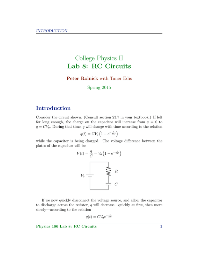
INTRODUCTION
College Physics II
Lab 8: RC Circuits
Peter Rolnick with Taner Edis
Spring 2015
Introduction
Consider the circuit shown. (Consult section 23.7 in your textbook.) If left
for long enough, the charge on the capacitor will increase from q = 0 to
q = CV0 . During that time, q will change with time according to the relation
t
q(t) = CV0 1 − e− RC
while the capacitor is being charged. The voltage difference between the
plates of the capacitor will be
t
q
= V0 1 − e− RC
V (t) =
C
X
X
X
X
X
X
X
X
V0
R
C
If we now quickly disconnect the voltage source, and allow the capacitor
to discharge across the resistor, q will decrease—quickly at first, then more
slowly—according to the relation
t
q(t) = CV0 e− RC
Physics 186 Lab 8: RC Circuits
1
ACTIVITY 1: THE RC CIRCUIT
while being discharged, and the voltage difference between the plates of the
capacitor will be
t
q
= V0 e− RC
V (t) =
(1)
C
X
X
X
X
X
X
X
X
R
C
This is what you will observe on the oscilloscope as we alternately charge
and discharge the capacitor. This is accomplished by using a square wave
voltage, which is equivalent to attaching and disconnecting a battery: when
in square wave mode, the function generator alternates between V = V0
and V = 0. The capacitor will charge when the square wave is at V = V0 ,
discharge when the square wave is at V = 0, charge, discharge, . . .
Activity 1: The RC Circuit
First, you will see a capacitor in an RC circuit charging and discharging,
and directly compare what you see with the voltage source which is being
turned on and off. For the set-up we will be using, the time to charge and
discharge is so fast that the only way you can see it is using an oscilloscope.
You will observe how the shape of the charging and discharging curves vary
as a function of the resistance in the circuit. You will also see that if you
don’t give the circuit enough time between when the voltage source turns on
and off, the circuit will not have time to completely charge or to completely
discharge, resulting in a decrease in amplitude.
Second, you will take measurements directly off the discharge curve on
the oscilloscope, and use those data to make a graph, the slope of which
is −1/RC. You will also calculate −1/RC using the nominal values of the
resistor and the capacitor, and compare that with your results from the
graph.
Physics 186 Lab 8: RC Circuits
2
ACTIVITY 1: THE RC CIRCUIT
X
X
X
X
X
X
X
X
f gen
R
C
Ch1 Ch2
Oscilloscope
Set up the circuit shown. The oscilloscope should be set to view both
traces; be sure you know which trace is which voltage: Ch1 is the function
generator and Ch2 is the capacitor. Set the function generator to square
wave, about 1000 Hz, and any voltage greater than zero. The R shown in
the diagram is actually a series combination of the external resistance (the
decade resistance box) and the internal resistance of the function generator
R = Rexternal + Rinternal
Rinternal = 600 Ω for the Pasco and Hewlett-Packard function generators,
Rinternal = 50.0 Ω for the Tektronix function generators. The capacitor is
.0100 µF, that is, 1.00 × 10−8 F.
Some precautions so the equipment survives:
• Make sure that the power supply is set on the 2 V peak-to-peak range.
The 20 V range could result in too much power dissipation—more than
the power rating of some of the circuit elements.
• Never allow any current to flow through the variable resistor when it
is set to zero resistance. Again, this could result in too much power
dissipation—more than the power rating of some of the components of
the variable resistor.
• Make sure that the negative (or ground) connections from Ch1 and Ch2
both go to the same point between the signal generator and the capacitor. Otherwise, you will have a ground loop problem. The negatives of
both Ch1 and Ch2 are connected to each other inside the oscilloscope,
so they must be connected to the same place in the circuit.
Physics 186 Lab 8: RC Circuits
3
ACTIVITY 1: THE RC CIRCUIT
Now, do the following:
1. Draw a picture of the Ch1 trace as compared to the Ch2 trace for a
range of values for R from 3000 Ω to 15,000 Ω, noting the difference
and similarities between the two traces for different values of R.
2. Notice, for a given set of values for R, C, and signal amplitude, what
happens to the Ch2 trace as the frequency gets very high. At very high
frequencies there should be hardly any amplitude. Ask yourself why.
Make a rough estimate of the frequencies at which the amplitude is
about 90% of the original, and where it is 10% of the original.
3. For a value of R where it looks like you get a nicely visible exponential
decay curve, turn off Ch1 and make the trace of Ch2 as large as possible.
Call the peak value V0 (t = 0 when V = V0 ), and as the voltage
decays, the value of V will become an increasingly smaller fraction of
V0 . Record about 5 to 10 points along the decay curve (not the charging
curve!) from V = V0 to V very near zero. Your data points should not
be evenly spaced along the horizontal axis; choose more of the points
from the region of the curve where V is changing at the greatest rate.
Since you are interested in values of V /V0 and not V , you do not have
to measure the vertical axis of the oscilloscope in Volts—number of
divisions will be fine. However, measurements off the horizontal axis
of the oscilloscope must be in seconds. To get a value for −1/RC
from these data, we need to consider the exponential decay expressed
in equation (1). With a little algebra, we get:
ln
V
V0
=−
t
RC
This means that if you graph ln(V /V0 ) (vertical on your graph) versus
t (horizontal), you will get a line with slope −1/RC. Don’t forget to
include the internal resistance in your data and calculations. See how
your result for −1/RC compares with that calculated directly from the
nominal values of the resistor and capacitor. Be sure you make this
graph and analyze it before you leave the lab.
Physics 186 Lab 8: RC Circuits
4
POSTSCRIPT
To hand in for activity 1
• Qualitative drawings of Ch1 and Ch2 traces, noting R = Rexternal +
Rinternal for each drawing.
• Rough experimental estimate of frequency at which amplitude in Ch2
noticeably decreases, and explanation.
• all data (Rinternal , Rexternal , C; V and V0 (in numbers of vertical divisions), t (in seconds),
• all quantities initially calculated from those data: R, t (in s), ln(V /V0 ),
• graph of ln(V /V0 ) versus t, and the slope of that graph,
• comparison of slope of above graph with −1/RC, using nominal values.
Postscript
As you can see from this lab, the oscilloscope can be used to find both
qualitative and quantitative details of a circuit. It might be used to troubleshoot a broken television set, or a broken component of a stereo system, by
looking at a portion of the circuit and seeing if it is behaving the way it is
supposed to.
You also noticed that an RC circuit will not respond to a periodic signal
if the frequency is significantly higher than 1/RC. Thus an RC circuit is
sometimes called a low pass filter, since it blocks high frequency signals.
Such a circuit might be useful if you wanted to filter out high frequency
static from a radio signal.
Physics 186 Lab 8: RC Circuits
5