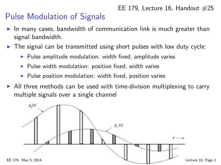
EE 179, Lecture 16, Handout #25
Pulse Modulation of Signals
◮
◮
◮
In many cases, bandwidth of communication link is much greater than
signal bandwidth.
The signal can be transmitted using short pulses with low duty cycle:
◮
Pulse amplitude modulation: width fixed, amplitude varies
◮
Pulse width modulation: position fixed, width varies
◮
Pulse position modulation: width fixed, position varies
All three methods can be used with time-division multiplexing to carry
multiple signals over a single channel
EE 179, May 5, 2014
Lecture 16, Page 1
PAM, PWM, PPM: Amplitude, Width, Position
EE 179, May 5, 2014
Lecture 16, Page 2
Pulse Amplitude Modulation
◮
The input to a pulse amplitude modulator is the real-world sample
of g(t):
Z Ts
q(t)g(t − nTs ) dt
g1 (nTs ) =
0
where q(t) is an integrator function. (Width of q(t) should be ≪ Ts .)
◮
Each transmitted pulse is narrow with height (or area) proportional
to g1 (nTs ). The pulse is integrated to obtain an analog value.
Z Tp
q1 (t)g1 (t − nTs ) dt
g̃(nTs ) =
0
where Tp ≪ Ts
◮
The original signal g(t) is reconstructed using an equalizer and a low
pass filter, as discussed in previous lecture.
EE 179, May 5, 2014
Lecture 16, Page 3
Pulse Width Modulation (PWM)
Pulse width modulation is also called pulse duration modulation (PDM).
PWM is more often used for control than for communication
◮
Motors (e.g., Apple II floppy disk drive)
◮
LEDs: output limunosity is proportional to average current.
◮
Galley slaves?
A signal can be recovered exactly from its PWM samples at rate 2B,
provided the bandwidth is ≤ 0.637B.
J. Huang, K. Padmanabhan, O. M. Collins, IEEE Trans. Circuits and Systems, 2011.
EE 179, May 5, 2014
Lecture 16, Page 4
PWM (cont.)
PWM output can be generated by a sawtooth signal gating the input.
Below the pulse width varies from nearly 0 to 1/2 the pulse period.
1
0.5
0
−0.5
−1
0
0.1
0.2
0.3
0.4
0.5
0.6
0.7
0.8
0.9
1
0
0.1
0.2
0.3
0.4
0.5
0.6
0.7
0.8
0.9
1
1
0.8
0.6
0.4
0.2
0
−0.2
EE 179, May 5, 2014
Lecture 16, Page 5
Pulse Position Modulation (PPM)
The value of the signal determines the delay of the pulse from the clock.
Electrical circuits use timers such as 555.
Microcontrollers can generate PPM (and PWM) in software.
(Counter-timer circuits (CTCs) were created for these applications.)
EE 179, May 5, 2014
Lecture 16, Page 6
Analog vs. Digital Communication
◮
Analog communication (baseband and modulated) is subject to noise.
◮
Pulse modulations (PAM, PWM, PPM) represent analog signals by
analog variations in pulses and are also sunbject to noise.
◮
Long distance communication requires repeaters, which amplify signal
and noise. Each link adds noise.
◮
Digital communication suppresses noise by regenerating signal.
EE 179, May 5, 2014
Lecture 16, Page 7
Pulse Code Modulation (PCM)
In PCM, a signal value is represented by a sequence of pulses (digits).
Width and spacing of pulses is constant. Value of pulse is chosen from a
small number of values.
Usually PCM uses only two pulse values, which represent 0 and 1.
If m bits are used, then 2m signal values can be represented.
◮
◮
◮
unsigned linear: 0, ν, . . . , ∆ν(2m − 1)
two’s complement: −∆ν2m−1 , . . . , ∆ν(2m−1 − 1)
A-law and µ-law: approximately logarithmic (more dynamic range)
EE 179, May 5, 2014
Lecture 16, Page 8
PCM and Quantization
Quantization of a signal produces the closest representable value.
For fixed number of values, spacing between values increases with range.
EE 179, May 5, 2014
Lecture 16, Page 9
PCM Tradeoffs
◮
Signal bandwidth determines minimum sample rate
◮
Desired signal fidelity determines precision of reproduced signal
◮
Signals can be quantized using digital-to-analog converter (DAC)
2
1
0
−1
−2
0
0.5
1
1.5
2
2.5
3
3.5
4
0
0.5
1
1.5
2
2.5
3
3.5
4
0
0.5
1
1.5
2
2.5
3
3.5
4
2
1
0
−1
−2
2
1
0
−1
−2
EE 179, May 5, 2014
Lecture 16, Page 10
Uniform Quantization
An ideal uniform quantizer is a nonlinear time invariant system:



−Nl ∆ν g(t) < −Nl ∆ν
ge(t) = n∆ν
(n − 21 )∆ν < g(t) < (n + 12 )∆ν, −Nl < n < Nh


N ∆ν
g(t) > N ∆ν
h
h
∆ν is quantization interval. Nl + Nh is number of levels.
EE 179, May 5, 2014
Lecture 16, Page 11
Nonuniform Quantization
Nonuniform quantizers increase quantization intervals as magnitude of
value. Interval proportional to value implies logarithmic curve.
An analog compressor (semiconductor diode) can be used.
EE 179, May 5, 2014
Lecture 16, Page 12
Nonuniform Quantization (cont.)
Logarithmic compression can be approximated by floating point, A-law, and
µ-law representations.
◮
Binary floating point corresponds to scientific notation:
±f × 2e
where f is significand or fraction and e is exponent. Both f and e are
represented in unsigned binary.
Example: 8-bit code with one bit for sign, 4 bits for f , 3 bits for e,
f = 0, 1, . . . , 15 ,
e = 0, 1, . . . , 7
The representable values range from −15 · 27 = −1920 to 1920.
Quantization spacing range from 1 for |y| < 16 to 128 for |y| > 960.
Disadvantage of floating point is that many values have multiple
representations. E.g., this scheme represents only 72 values.
Some writers use mantissa instead of significand.
EE 179, May 5, 2014
Lecture 16, Page 13
Nonuniform Quantization (cont.)
Telephone systems use ITU standardized compression formula.
◮ µ-law: North America and Japan. For µ = 255 (for 8-bit codes),
1
ln (1 + |x|) , (0 < x < 1)
ln(1 + µ)
A-law: Europe, rest of world.

A|x|
1


|x| <
sgn(x) 1 + ln(A)
A
y=

1 + ln(A|x|) 1

sgn(x)
< |x| < 1
y = sgn(x)
◮
1 + ln(A)
A
The standard value is A = 87.7.
For both laws, the input to the compressor is
x=
where −mp ≤ m(t) ≤ mp .
EE 179, May 5, 2014
m(t)
mp
Lecture 16, Page 14
Comparison of µ-Law and A-Law
◮
µ-law provides slightly larger dynamic range than A-law.
◮
A-law has smaller proportional distortion for small signals.
◮
A-law is used for international connections if at least one country uses it.
EE 179, May 5, 2014
Lecture 16, Page 15
µ-Law Implementation
Both µ-law and A-law expanders are piecewise linear.
This table shows how 7 bits are expanded.
In practice this table is used by the µ-law encoder.
EE 179, May 5, 2014
Lecture 16, Page 16
µ-Law Signal-to-Noise Ratio
The average power of a compressed signal is closer to the peak power.
EE 179, May 5, 2014
Lecture 16, Page 17
Examples of Continuous Random Variables (cont.)
Gaussian random variable has two parameters µ and σ. Its pdf is
1
(x − µ)2
2
N (x; µ, σ ) = √
exp −
σ2
2πσ 2
The Gaussian PDF is centered at and has maximum value at x = µ.
The mean is µ (obvious) and the variance is σ 2 .
The inflection points of the density graph are at ±σ.
The density decreases faster than exponentially as x → ±∞.
EE 179, May 5, 2014
Lecture 16, Page 18
Gaussian Noise Example
EE 179, May 5, 2014
Lecture 16, Page 19