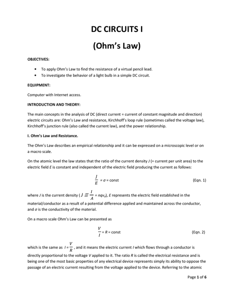
DC CIRCUITS I
(Ohm’s Law)
OBJECTIVES:
•
•
To apply Ohm’s Law to find the resistance of a virtual pencil lead.
To investigate the behavior of a light bulb in a simple DC circuit.
EQUIPMENT:
Computer with Internet access.
INTRODUCTION AND THEORY:
The main concepts in the analysis of DC (direct current = current of constant magnitude and direction)
electric circuits are: Ohm’s Law and resistance, Kirchhoff’s loop rule (sometimes called the voltage law),
Kirchhoff’s junction rule (also called the current law), and the power relationship.
I. Ohm’s Law and Resistance.
The Ohm’s Law describes an empirical relationship and it can be expressed on a microscopic level or on
a macro scale.
On the atomic level the law states that the ratio of the current density J (= current per unit area) to the
electric field E is constant and independent of the electric field producing the current as follows:
!
"
where J is the current density ( J
= σ = const
(Eqn. 1)
$
= nqvd), E represents the electric field established in the
%
material/conductor as a result of a potential difference applied and maintained across the conductor,
and σ is the conductivity of the material.
On a macro scale Ohm’s Law can be presented as
&
$
which is the same as I =
= R = const
(Eqn. 2)
&
, and it means the electric current I which flows through a conductor is
'
directly proportional to the voltage V applied to it. The ratio R is called the electrical resistance and is
being one of the most basic properties of any electrical device represents simply its ability to oppose the
passage of an electric current resulting from the voltage applied to the device. Referring to the atomic
Page 1 of 6
level the electrical resistance of an object arises from the random collisions between the free electrons
carrying the current with fixed atoms of the material. This repeated process causes scattering of the
electrons and makes them drift in the direction opposite that of the internal electric field. If V is in Volts
and I is in Amperes, R is in ohms, Ω.
Materials which have a constant resistance over a considerable range of applied voltages or currents for
a given temperature are said to be ohmic. For such materials/devices the plot of I vs. V (usually called
the “I-V characteristic”) is a straight line passing through the origin and the reciprocal of the slope
represents the resistance of the device. Ohmic objects with a very low resistance and thus being able to
transfer current with the least loss of electrical energy are called conductors. Example: electrical wires.
Materials that have non-linear I-V curve, which resistance changes with voltage or current, are called
non-ohmic. Example: semiconductor diodes, transistors.
I (A)
I (A)
R=
*
,-./0
= constant
V (V)
V (V)
(a)
(b)
Fig. 1. A sample current-voltage characteristic for an ohmic (a)
and a non-ohmic (b) device.
The resistance of a given ohmic conductor increases with length and decreases for larger crosssectional area. For a conductor of uniform cross section A and length ( the resistance R can be
computed as:
R=ρ
)
%
,
(Eqn. 3)
where the proportionality constant ρ is the electrical resistivity of the material measured in ohmmeters, Ωm. While the resistance of a device depends on its geometry, the resistivity is specific
for the material used in the device and depends on the nature of the material and on temperature
*
but not on its shape or size. The resistivity is the inverse of conductivity ρ = . For all metals
+
Page 2 of 6
resistivity increases with temperature. For conductors the resistivity changes approximately
linearly with temperature over a limited range of temperature according to the following formula
ρ = ρo [1 + α (T- T0)],
(Eqn. 4)
where ρ is the resistivity at temperature T (in ºC), ρo is the resistivity at some reference
temperature T0 (usually 20º C), and α is called the temperature coefficient of resistivity expressed
*
in
. Since resistance is proportional to resistivity a similar expression is true for the resistance
°2
dependence on temperature:
R = R0 [1 + α (T – T0)]
(Eqn. 5)
PROCEDURE
Part 1. Determining the resistance of a pencil lead.
The Ohm’s law can be used to find electrical properties, namely the resistance, of any conductor. In this
part of the experiment you will apply the Ohm’s Law to determine the resistance of a virtual pencil lead.
You will measure the current through the pencil lead and the voltage drop across this element for a few
output voltages delivered by the battery. Next, you will present the data graphically, plotting I PENCIL vs.
v PENCIL, and analyze the plot to find the resistance of the simulated pencil.
Open the PhET Interactive Simulations web page http://phet.colorado.edu/en/simulation/circuitconstruction-kit-dc-virtual-lab and download the Circuit Construction Kit (DC Only), Virtual Lab. Using
the circuit components from the right tool menus and the Grab Bag options (that is where you find the
pencil lead) construct the circuit similar to the one shown in Fig.2. Please, note that the ammeter is
connected in series with the pencil while the voltmeter leads are attached to the pencil tips in parallel
fashion (the red lead of the meter touches the pencil end of the higher potential and the black lead is
connected to the end of the lower potential).
Page 3 of 6
,
Fig. 2. Circuit for measuring the resistance of the pencil lead.
Right click on the battery allows you to select the Voltage Change option which opens the voltage
selection window as seen in Fig.2. For your convenience, please, leave this window open for easy access.
By adding the internal resistance of the battery we will make this circuit behaving even more life-like –
right click on the battery again and change its internal resistance to 9 Ω. Apply 5 different voltages from
the battery, ranging from 0 to 100 Volts and evenly spread. After adjusting the battery voltage to the
desired value, close the switch and record the current measured by the ammeter, I PENCIL , and the
voltage detected by the voltmeter, V PENCIL.
Open the LoggerPro program available in MyApps on My ASU site. The default screen contains a twocolumn data table and a graph window. Enter the V PENCIL data (expressed in Volts, V) in the first column,
and the I PENCIL values (expressed in Amperes, A) in the second column. Double click the heading of each
column to change its name (X → V, Y → I), enter the units for the typed-in data and select the number of
decimal places you wish to be displayed. Create a new calculated column for the resistance R expressed
in ohms, Ω.
Hint: To add a calculated column to the data table select “Data” in the upper tool bar options, and then
“New Calculated Column…”. In the equation field type “V”/”I”, where V and I should be chosen from the
pull down Variables selection.
After entering the experimental data in the table you should automatically see them being plotted in the
graph window. As a good scientific habit you always want to show only the collected data points without
the lines in-between them. So, double click on the graph window and uncheck the option “Connect
Points”. Apply the linear fit to your set of data. Double click on the small window with the fit
parameters and select show uncertainty. From the slope calculate the resistance of the virtual pencil.
Propagate the uncertainty in the slope into the uncertainty of the experimental resistance of the pencil.
Page 4 of 6
Re-scale the whole graph window to about half of the available screen space, without covering the data
table. Insert a second graph displaying the resistance calculated in the third column on both axis of the
new graph. Again, uncheck the “Connect Points” option. Re-scale this graph window to fit into the space
remaining on the page. By dragging around with the mouse, select all data points of this plot and apply
statistics from the Analyze menu. Save the LoggerPro file for future reference. How does the mean value
displayed in the statistics window compare to the resistance computed from the slope of the first
graph? State the measured resistance of the virtual pencil lead along with its uncertainty. Remember to
express the uncertainty with just one (or maximum two) sig figure(s) and adjust the number of decimal
places in the main result appropriately. Based on your data conclude whether the virtual pencil was an
ohmic element or not.
Capture the screen with the LoggerPro file and paste it into MS Word – you will have to attach it to your
lab report. It is recommended to use the landscape orientation for the page layout in MS Word.
If you assume that the virtual pencil lead was made out of material of resistivity ρ = 3.5×10-4 Ωm (a
composition of graphite) and the diameter of the lead was 0.6 mm, how long was the pencil? On
average the real pencil rod has a diameter of 2.4 ± 0.1 mm and the length of 18.0 ± 0.1 cm. If it was
made of the same material as the virtual pencil what resistance would it have? Propagate the errors in
the dimension measurements into the final uncertainty of the calculated resistance.
Part 2. Investigating the resistive properties of a light bulb.
Using Firefox login to VirtualPhysicsLabs: http://virtuallabs.ket.org/physics/. Click the Labs tab and select
lab 16 -DC Circuits. Before running the simulation read the full description and detailed information.
Connect the circuit shown below. Make sure to keep the default setting for the wire resistance at 0 Ω.
Please, note that the ammeter must always be connected in series with the investigated object (the light
bulb in our case) to measure the current flowing through it, while the voltmeter is wired in parallel with
Page 5 of 6
the object to show the potential difference across it without disturbing the current distribution within
the circuit.
Click the battery and adjust its voltage to 1 V. Double click the switch to close the circuit. Open a new file
in LoggerPro and record the first pair of data: the voltage across the light bulb as measured by the
voltmeter and the current displayed by the ammeter. Remember to label the column headings
appropriately and enter the units. Since the internal resistance of the ammeter is negligible, there is no
potential drop across this instrument and the voltage across the light bulb equals the output voltage
from the battery. Next, open the switch. Change the battery output signal to 2 V, close the switch and
record the new values for the current and voltage of the light bulb. Open the switch and repeat the
same procedure for the following voltages from the battery: 4 V, 6 V, 8 V, 10 V, 20 V, 30 V, 40 V, 50 V
and 60 V. Add a new calculated column to the data table showing the resistance of the bulb, expressed
in Ω, as determined from Ohm’s law. Now, assuming that the filament of the bulb is made of tungsten
for which the temperature coefficient of resistivity is α = 4.5× 10-3 1/°C, and the resistance of the bulb at
T0= 20 °C is R0= 10 Ω, create yet another calculated column displaying the temperature of the bulb.
Hint: Rearrange eqn. 5 to get a direct relationship of T = f(R).
Insert a new graph showing the filament temperature T (Y-axis) vs. the filament resistance R(X-axis).
Apply the linear fit to your set of data of T vs. R. Re-size both graph windows (I vs. V and T vs. R) so they
nicely fit on one page along with the data table. Save your LogegrPro file for future reference.
Based on the graph of I vs. V for the light bulb what can you conclude: is the bulb an ohmic or a nonohmic circuit element?
Finally, calculate the ratio rR of the resistance of the bulb at 60 V to its resistance at 1 V. Also, compute a
similar ratio rT for the corresponding bulb temperatures. Which parameter: the filament resistance or its
temperature was increasing with a faster rate?
Capture the screen with the LoggerPro file and paste it into MS Word – you will have to attach it to your
lab report. It is recommended to use the landscape orientation for the page layout in MS Word.
* Include answers to all questions in lab report
Page 6 of 6