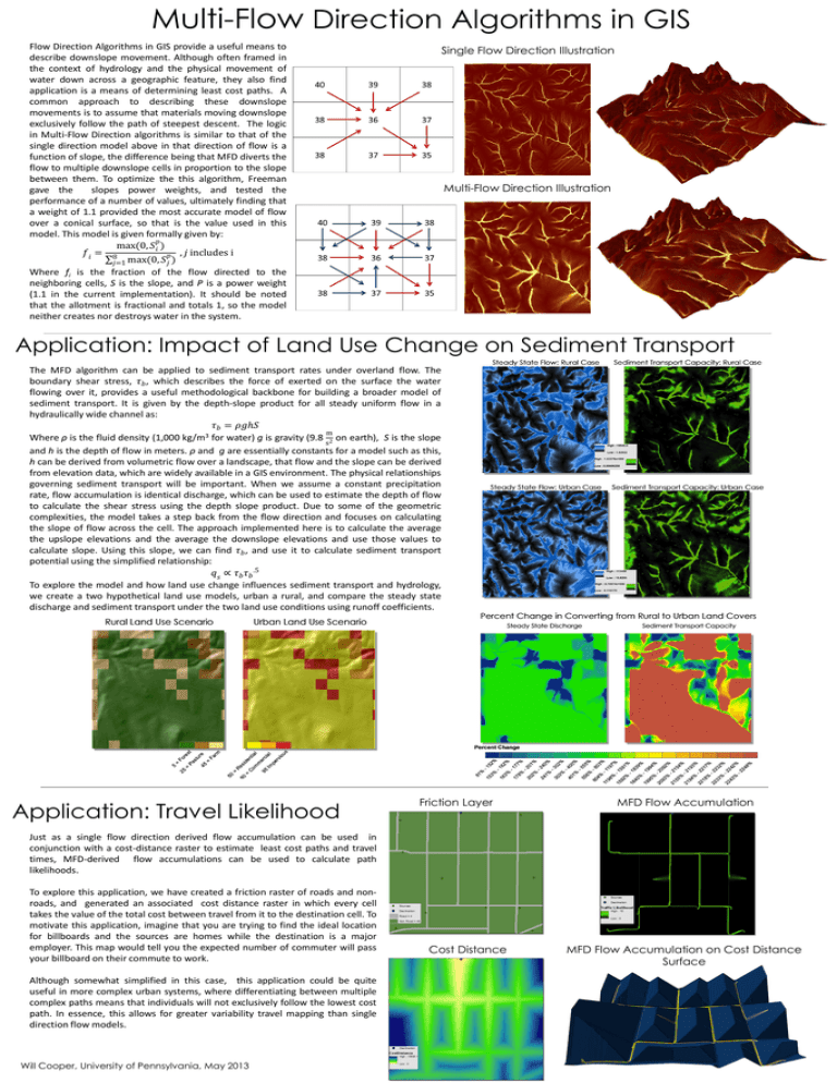
Multi-Flow Direction Algorithms in GIS
Flow Direction Algorithms in GIS provide a useful means to
describe downslope movement. Although often framed in
the context of hydrology and the physical movement of
water down across a geographic feature, they also find
application is a means of determining least cost paths. A
common approach to describing these downslope
movements is to assume that materials moving downslope
exclusively follow the path of steepest descent. The logic
in Multi-Flow Direction algorithms is similar to that of the
single direction model above in that direction of flow is a
function of slope, the difference being that MFD diverts the
flow to multiple downslope cells in proportion to the slope
between them. To optimize the this algorithm, Freeman
gave the
slopes power weights, and tested the
performance of a number of values, ultimately finding that
a weight of 1.1 provided the most accurate model of flow
over a conical surface, so that is the value used in this
model. This model is given formally given by:
𝑝
max(0, 𝑆𝑖 )
𝑓𝑖 = 8
𝑝 , 𝑗 includes i
𝑗=1 max(0, 𝑆𝑗 )
Where fi is the fraction of the flow directed to the
neighboring cells, S is the slope, and P is a power weight
(1.1 in the current implementation). It should be noted
that the allotment is fractional and totals 1, so the model
neither creates nor destroys water in the system.
Single Flow Direction Illustration
Multi-Flow Direction Illustration
Application: Impact of Land Use Change on Sediment Transport
The MFD algorithm can be applied to sediment transport rates under overland flow. The
boundary shear stress, 𝜏𝑏 , which describes the force of exerted on the surface the water
flowing over it, provides a useful methodological backbone for building a broader model of
sediment transport. It is given by the depth-slope product for all steady uniform flow in a
hydraulically wide channel as:
𝜏𝑏 = 𝜌𝑔ℎ𝑆
m
Where ρ is the fluid density (1,000 kg/m3 for water) g is gravity (9.8 s2 on earth), S is the slope
and h is the depth of flow in meters. ρ and g are essentially constants for a model such as this,
h can be derived from volumetric flow over a landscape, that flow and the slope can be derived
from elevation data, which are widely available in a GIS environment. The physical relationships
governing sediment transport will be important. When we assume a constant precipitation
rate, flow accumulation is identical discharge, which can be used to estimate the depth of flow
to calculate the shear stress using the depth slope product. Due to some of the geometric
complexities, the model takes a step back from the flow direction and focuses on calculating
the slope of flow across the cell. The approach implemented here is to calculate the average
the upslope elevations and the average the downslope elevations and use those values to
calculate slope. Using this slope, we can find 𝜏𝑏 , and use it to calculate sediment transport
potential using the simplified relationship:
𝑞𝑠 ∝ 𝜏𝑏 𝜏𝑏 .5
To explore the model and how land use change influences sediment transport and hydrology,
we create a two hypothetical land use models, urban a rural, and compare the steady state
discharge and sediment transport under the two land use conditions using runoff coefficients.
Application: Travel Likelihood
Friction Layer
MFD Flow Accumulation
Just as a single flow direction derived flow accumulation can be used in
conjunction with a cost-distance raster to estimate least cost paths and travel
times, MFD-derived flow accumulations can be used to calculate path
likelihoods.
To explore this application, we have created a friction raster of roads and nonroads, and generated an associated cost distance raster in which every cell
takes the value of the total cost between travel from it to the destination cell. To
motivate this application, imagine that you are trying to find the ideal location
for billboards and the sources are homes while the destination is a major
employer. This map would tell you the expected number of commuter will pass
your billboard on their commute to work.
Although somewhat simplified in this case, this application could be quite
useful in more complex urban systems, where differentiating between multiple
complex paths means that individuals will not exclusively follow the lowest cost
path. In essence, this allows for greater variability travel mapping than single
direction flow models.
Will Cooper, University of Pennsylvania, May 2013
Cost Distance
MFD Flow Accumulation on Cost Distance
Surface