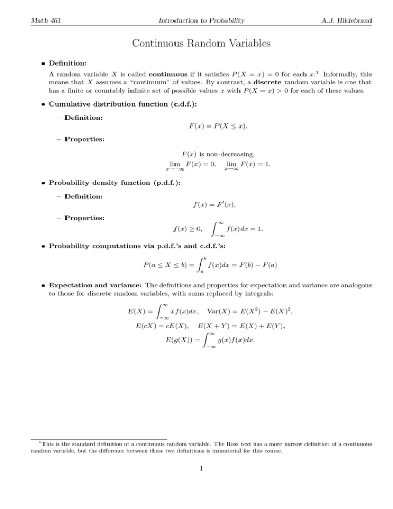
Math 461
Introduction to Probability
A.J. Hildebrand
Continuous Random Variables
• Definition:
A random variable X is called continuous if it satisfies P (X = x) = 0 for each x.1 Informally, this
means that X assumes a “continuum” of values. By contrast, a discrete random variable is one that
has a finite or countably infinite set of possible values x with P (X = x) > 0 for each of these values.
• Cumulative distribution function (c.d.f.):
– Definition:
F (x) = P (X ≤ x).
– Properties:
F (x) is non-decreasing,
lim F (x) = 0,
lim F (x) = 1.
x→∞
x→−∞
• Probability density function (p.d.f.):
– Definition:
f (x) = F 0 (x),
– Properties:
Z
∞
f (x) ≥ 0,
f (x)dx = 1.
−∞
• Probability computations via p.d.f.’s and c.d.f.’s:
Z
P (a ≤ X ≤ b) =
b
f (x)dx = F (b) − F (a)
a
• Expectation and variance: The definitions and properties for expectation and variance are analogous
to those for discrete random variables, with sums replaced by integrals:
Z ∞
E(X) =
xf (x)dx, Var(X) = E(X 2 ) − E(X)2 ,
−∞
E(cX) = cE(X),
E(X + Y ) = E(X) + E(Y ),
Z ∞
E(g(X)) =
g(x)f (x)dx.
−∞
1
This is the standard definition of a continuous random variable. The Ross text has a more narrow definition of a continuous
random variable, but the difference between these two definitions is immaterial for this course.
1
Math 461
Introduction to Probability
A.J. Hildebrand
• Notes and tips:
– Note that, although a p.d.f. f (x) of a continuous r.v. plays the same role as a p.m.f.
p(x) of a discrete r.v., the definitions of these two functions are completely different:
In the discrete case, p(x) is defined as p(x) = P (X = x). In the continuous case, the probabilities
P (X = x) are 0, so the same definition would not make sense; in fact, f (x) can only be obtained
indirectly as the derivative of the c.d.f. F (x).
Another difference between the functions f (x) and p(x) is that a p.d.f. f (x) can take values larger
than 1, while a p.m.f. p(x) always satisfies 0 ≤ p(x) ≤ 1.
– Keep track of the “range” of a density: Most random variables have a finite, or one-sided
infinite, range (i.e., set of values), such as the interval [0, 1], or [1, ∞). Outside this range the
density function f (x) is 0. It is important to keep this range in mind when trying to determine
the correct integration limits. For example, if a problem asks for P (X ≥ 2) and the density f (x)
“lives” on the interval [1, 4], the integral giving P (X ≥ 2) should be from 2 to 4; if, instead, f (x)
were defined and non-zero on the infinite interval [1, ∞), the integral would be from 2 to infinity.
To prevent mistakes, make it a habit to always write down the “range” of a density f (x) along
with the formula. i.e., the interval of x on which the function is defined and non-zero).
– For probabilities involving continuous random variables, “≤” and “<”, and similarly
“≥” and “>”, are interchangeable: For example, P (X ≤ 2) is the same as P (X < 2), since
the difference between these two probabilities, P (X = 2), is 0 for a continuous random variable.
By the same token, when specifying the range of a density functions, it doesn’t matter whether
or not one includes the boundary points in the range. For example, in the definition “f (x) = 2x
for 0 < x < 1” one could replace the range “0 < x < 1” by “0 ≤ x ≤ 1” without affecting any
probability calculations involving this density.
2