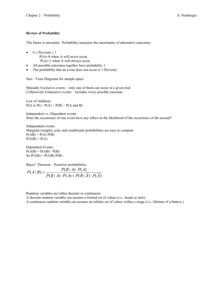
Chapter 2 – Probability
S. Neuburger
Review of Probability
The future is uncertain. Probability measures the uncertainty of alternative outcomes.



0 ≤ P(event) ≤ 1
P(A)=0 when A will never occur
P(A)=1 when A will always occur
All possible outcomes together have probability 1
The probability that an event does not occur is 1-P(event)
Sets - Venn Diagrams for sample space
Mutually Exclusive events – only one of them can occur in a given trial
Collectively Exhaustive events – includes every possible outcome
Law of Addition:
P(A or B) = P(A) + P(B) – P(A and B)
Independent vs. Dependent events
Does the occurrence of one event have any effect on the likelihood of the occurrence of the second?
Independent events:
Marginal (simple), join, and conditional probabilities are easy to compute
P(AB) = P(A) P(B)
P(A|B) = P(A)
Dependent Events:
P(A|B) = P(AB) / P(B)
So P(AB) = P(A|B) P(B)
Bayes’ Theorem – Posterior probabilities
P( A | B) 
P( B | A)  P( A)
P( B | A)  P( A)  P( B | A )  P( A )
Random variables are either discrete or continuous:
A discrete random variable can assume a limited set of values (i.e., heads or tails).
A continuous random variable can assume an infinite set of values within a range (i.e., lifetime of a battery.)
Chapter 2 – Probability
S. Neuburger
Measures of Central tendency
Sample Mean
X 
1 n
 Xi
n i 1
Mean (or Expected Value)
n
μ = E(X) =
X
i 1
i
 P( X i )
Variance reveals overall spread of distribution
n
σ2 =
[ X
i 1
i
 E ( X )] 2  P( X i )
Standard deviation = square root of variance
  2
Probability Distributions:
Binomial – only 2 possible outcomes in each independent trial (success and failure)
B(n,p) where n=sample size and p=probability of success
P(k) = P(k successes) =
 p
n
k
k
(1  p ) n k
Normal – Symmetric, bell-shaped curve; many variables in real life are normally distributed and reasonable
approximation for other distributions.
To convert N(μ ,σ) to N(0, 1), which is the standard normal distribution use Z=(x- μ)/ σ
Exponential – continuous
f(x) =
 e  x
Poisson - discrete
P(x) =
x e 
x!