Matrix Algebra and R
1
Matrices
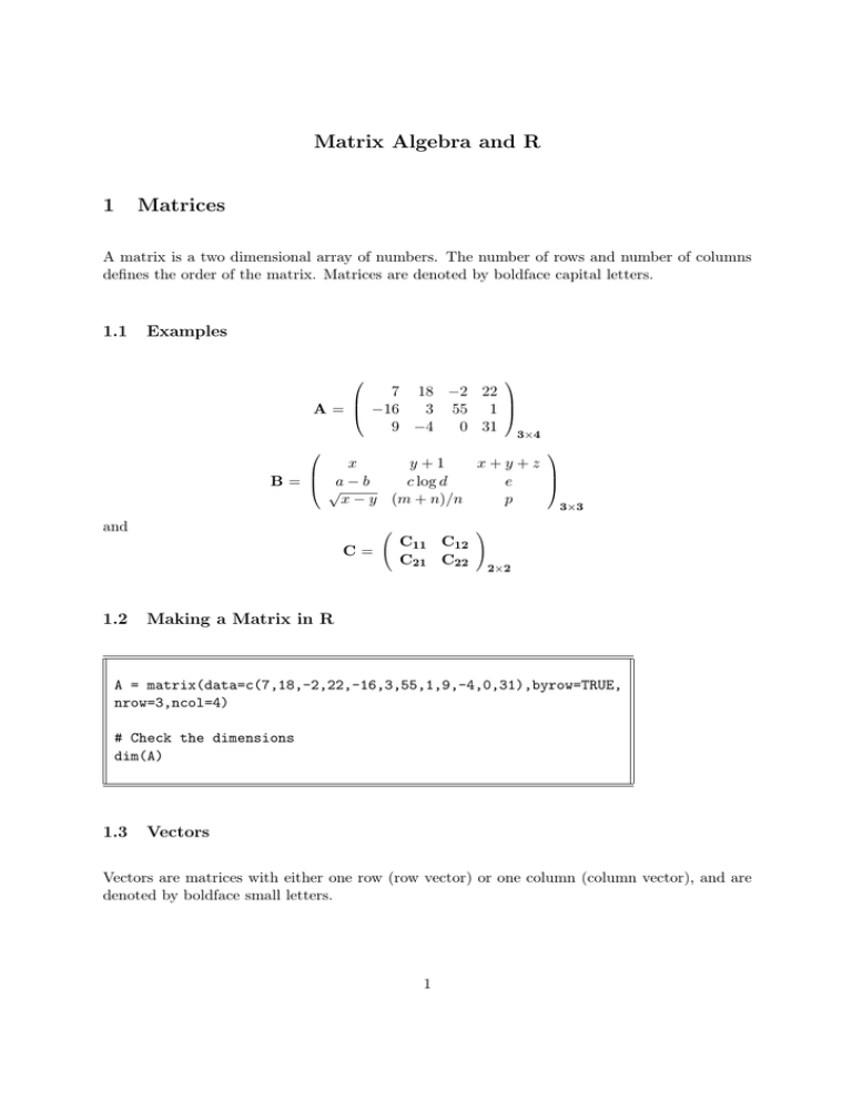
A matrix is a two dimensional array of numbers. The number of rows and number of columns
defines the order of the matrix. Matrices are denoted by boldface capital letters.
1.1
Examples


7 18 −2 22


3 55 1 
A =  −16
9 −4
0 31 3×4


x
y+1
x+y+z


c log d
e
B =  a−b

√
x − y (m + n)/n
p
3×3
and
C=
1.2
C11 C12
C21 C22
!
2×2
Making a Matrix in R
A = matrix(data=c(7,18,-2,22,-16,3,55,1,9,-4,0,31),byrow=TRUE,
nrow=3,ncol=4)
# Check the dimensions
dim(A)
1.3
Vectors
Vectors are matrices with either one row (row vector) or one column (column vector), and are
denoted by boldface small letters.
1
1.4
Scalar
A scalar is a matrix with just one row and one column, and is denoted by an letter or symbol.
2
Special Matrices
2.1
Square Matrix
A matrix with the same number of rows and columns.
2.2
Diagonal Matrix
Let {aij } represent a single element in the matrix A. A diagonal matrix is a square matrix in
which all aij are equal to zero except when i equals j.
2.3
Identity Matrix
This is a diagonal matrix with all aii equal to one (1). An identity matrix is usually written as
I.
To make an identity matrix with r rows and columns, use
id = function(n) diag(c(1),nrow=n,ncol=n)
# To create an identity matrix of order 12
I12 = id(12)
2.4
J Matrix
A J matrix is a general matrix of any number of rows and columns, but in which all elements
in the matrix are equal to one (1).
The following function will make a J matrix, given the number or rows, r, and number of
columns, c.
2
jd = function(n,m) matrix(c(1),nrow=n,ncol=m)
# To make a matrix of 6 rows and 10 columns of all ones
M = jd(6,10)
2.5
Null Matrix
A null matrix is a J matrix multiplied by 0. That is, all elements of a null matrix are equal to
0.
2.6
Triangular Matrix
A lower triangular matrix is a square matrix where elements with j greater than i are equal to
zero (0), { aij } equal 0 for j greater than i. There is also an upper triangular matrix in which
{aij } equal 0 for i greater than j.
2.7
Tridiagonal Matrix
A tridiagonal matrix is a square matrix with all elements equal to zero except the diagonals and
the elements immediately to the left and right of the diagonal. An example is shown below.





B= 



10 3 0 0 0 0
3 10 3 0 0 0
0 3 10 3 0 0
0 0 3 10 3 0
0 0 0 3 10 3
0 0 0 0 3 10
3





.



3
Matrix Operations
3.1
Transposition
Let {aij } represent a single element in the matrix A. The transpose of A is defined as
A0 = {aji }.
If A has r rows and c columns, then A0 has c rows and r columns.


7 18 −2 22


3 55 1 
A =  −16
9 −4
0 31




A0 = 

7 −16
9
18
3 −4 

.
−2
55
0 
22
1 31
In R,
At = t(A)
# t() is the transpose function
3.2
Diagonals
The diagonals of matrix A are {aii } for i going from 1 to the number of rows in the matrix.
Off-diagonal elements of a matrix are all other elements excluding the diagonals.
Diagonals can be extracted from a matrix in R by using the diag() function.
3.3
Addition of Matrices
Matrices are conformable for addition if they have the same order. The resulting sum is a matrix
having the same number of rows and columns as the two matrices to be added. Matrices that
4
are not of the same order cannot be added together.
A = {aij } and B = {bij }
A + B = {aij + bij }.
An example is
A=
4 5 3
6 0 2
!
and B =
1 0 2
3 4 1
then
A+B =
=
4+1 5+0 3+2
6+3 0+4 2+1
5 5 5
9 4 3
!
!
!
= B + A.
Subtraction is the addition of two matrices, one of which has all elements multiplied by a
minus one (-1). That is,
!
3
5 1
.
A + (−1)B =
3 −4 1
R will check matrices for conformability, and will not perform the operation unless they are
conformable.
3.4
Multiplication of Matrices
Two matrices are conformable for multiplication if the number of columns in the first matrix
equals the number of rows in the second matrix.
If C has order p × q and D has order m × n, then the product CD exists only if q = m. The
product matrix has order p × n.
In general, CD does not equal DC, and most often the product DC may not even exist
because D may not be conformable for multiplication with C. Thus, the ordering of matrices
in a product must be carefully and precisely written.
The computation of a product is defined as follows: let
Cp×q = {cij }
and
Dm×n = {dij }
5
and q = m, then
CDp×n = {
m
X
cik dkj }.
k=1
As an example, let




1
1
6 4 −3




0 ,
C =  3 9 −7  and D =  2
3 −1
8 5 −2
then




5 9
6(1) + 4(2) − 3(3) 6(1) + 4(0) − 3(−1)




CD =  3(1) + 9(2) − 7(3) 3(1) + 9(0) − 7(−1)  =  0 10  .
12 10
8(1) + 5(2) − 2(3) 8(1) + 5(0) − 2(−1)
In R,
# C times D - conformability is checked
CD = C %*% D
3.4.1
Transpose of a Product
The transpose of the product of two or more matrices is the product of the transposes of each
matrix in reverse order. That is, the transpose of CDE, for example, is E0 D0 C0 .
3.4.2
Idempotent Matrix
A matrix, say A, is idempotent if the product of the matrix with itself equals itself, i.e. AA = A.
This implies that the matrix must be square, but not necessarily symmetric.
3.4.3
Nilpotent Matrix
A matrix is nilpotent if the product of the matrix with itself equals a null matrix, i.e. BB = 0,
then B is nilpotent.
6
3.4.4
Orthogonal Matrix
A matrix is orthogonal if the product of the matrix with its transpose equals an identity matrix,
i.e. UU0 = I, which also implies that U0 U = I.
3.5
Traces of Square Matrices
The trace is the sum of the diagonal elements of a matrix. The sum is a scalar quantity. Let


.51 −.32 −.19


.46 −.14  ,
A =  −.28
−.21 −.16
.33
then the trace is
tr(A) = .51 + .46 + .33 = 1.30.
In R, the trace is achieved using the sum() and diag() functions together. The diag()
function extracts the diagonals of the matrix, and the sum() function adds them together.
# Trace of the matrix A
trA = sum(diag(A))
3.5.1
Traces of Products - Rotation Rule
The trace of the product of conformable matrices has a special property known as the rotation
rule of traces. That is,
tr(ABC) = tr(BCA) = tr(CAB).
The traces are equal, because they are scalars, even though the dimensions of the three products
might be greatly different.
3.6
Euclidean Norm
The Euclidean Norm is a matrix operation usually used to determine the degree of difference
between two matrices of the same order. The norm is a scalar and is denoted as kAk .
0 .5
kAk = [tr(AA )] = (
n X
n
X
i=1 j=1
7
a2ij ).5 .
For example, let


7 −5 2


6 3 ,
A=  4
1 −1 8
then
kAk = (49 + 25 + 4 + · · · + 1 + 64).5
= (205).5 = 14.317821.
Other types of norms also exist.
In R,
# Euclidean Norm
EN = sqrt(sum(diag(A %*% t(A))))
3.7
Direct Sum of Matrices
For matrices of any dimension, say H1 , H2 , . . . Hn , the direct sum is

P+
i


Hi = H1 ⊕ H2 ⊕ · · · ⊕ Hn = 


H1
0
..
.
0
0
··· 0
H2 · · · 0
..
. . ..
. .
.
0
· · · Hn



.


In R, the direct sum is accomplished by the block() function which is shown below.
8
# Direct sum operation via the block function
block <- function( ... ) {
argv = list( ... )
i = 0
for( a in argv ) {
m = as.matrix(a)
if(i == 0)
rmat = m
else
{
nr = dim(m)[1]
nc = dim(m)[2]
aa = cbind(matrix(0,nr,dim(rmat)[2]),m)
rmat = cbind(rmat,matrix(0,dim(rmat)[1],nc))
rmat = rbind(rmat,aa)
}
i = i+1
}
rmat
}
To use the function,
Htotal = block(H1,H2,H3,H4)
3.8
Kronecker Product
The Kronecker product, also known as the direct product, is where every element of the first
matrix is multiplied, as a scalar, times the second matrix. Suppose that B is a matrix of order
m × n and that A is of order 2 × 2, then the direct product of A times B is
A⊗B =
a11 B a12 B
a21 B a22 B
!
.
Notice that the dimension of the example product is 2m × 2n.
In R, a direct product can be obtained as follows:
9
AB = A %x% B
# Note the small x between % %
3.9
Hadamard Product
The Hadamard product exists for two matrices that are conformable for addition. The corresponding elements of the two matrices are multiplied together. The order of the resulting
product is the same as the matrices in the product. For two matrices, A and B of order 2 × 2,
then the Hadamard product is
AB =
a11 b11 a12 b12
a21 b21 a22 b22
In R,
AB = A * B
10
!
.
4
Elementary Operators
Elementary operators are identity matrices that have been modified for a specific purpose.
4.1
Row or Column Multiplier
The first type of elementary operator matrix has one of the diagonal elements of an identity
matrix replaced with a constant other than 1. In the following example, the {1,1} element has
been set to 4. Note what happens when the elementary operator is multiplied times the matrix
that follows it.





4 8 12 16
1 2 3 4
4 0 0





7 6 5 .
8
7
6
5
0
1
0
=

 8


9 10 11 12
9 10 11 12
0 0 1
4.2
Interchange Rows or Columns
The second type of elementary operator matrix interchanges rows or columns of a matrix. To
change rows i and j in a matrix, the identity matrix is modified by interchange rows i and j, as
shown in the following example. Note the effect on the matrix that follows it.





1 2 3 4
1 2 3 4
1 0 0





7 6 5  =  9 10 11 12  .
 0 0 1  8
8 7 6 5
9 10 11 12
0 1 0
4.3
Combine Two Rows
The third type of elementary operator is an identity matrix that has an off-diagonal zero element
changed to a non-zero constant. An example is given below, note the effect on the matrix that
follows it.





1 0 0
1 2 3 4
1 2 3 4





7 6 5  =  7 5 3 1 .
 −1 1 0   8
0 0 1
9 10 11 12
9 10 11 12
11
5
Matrix Inversion
An inverse of a square matrix A is denoted by A−1 . An inverse of a matrix pre- or postmultiplied times the original matrix yields an identity matrix. That is,
AA−1 = I, and A−1 A = I.
A matrix can be inverted if it has a nonzero determinant.
5.1
Determinant of a Matrix
The determinant of a matrix is a single scalar quantity. For a 2 × 2 matrix, say
a11 a12
a21 a22
A=
!
,
then the determinant is
|A| = a11 a22 − a21 a12 .
For a 3 × 3 matrix, the determinant can be reduced to a series of determinants of 2 × 2 matrices.
For example, let


6 −1
2


4 −5  ,
B=  3
1
0 −2
then
4 −5
|B| = 6 0 −2
3 −5
− 1(−1) 1 −2
3 4
+ 2
1 0
= 6(−8) + 1(−1) + 2(−4)
= − 57.
The general expression for the determinant of a matrix is
|B| =
n
X
(−1)i+j bij |Mij |
j=1
where B is of order n, and Mij is a minor submatrix of B resulting from the deletion of the ith
row and j th column of B. Any row of B may be used to compute the determinant because the
result should be the same for each row. Columns may also be used instead of rows.
In R, the det() function may be used to compute the determinant.
12
5.2
Matrix of Signed Minors
If the determinant is non-zero, the next step is to find the matrix of signed minors, known as
the adjoint matrix. Using the same matrix, B above, the minors and their determinants are
as follows:
!
M11 = +1
4 −5
0 −2
!
M12 = −1
3 −5
1 −2
M13 = +1
3 4
1 0
M21 = −1
−1
2
0 −2
!
M22 = +1
6
2
1 −2
!
M23 = −1
6 −1
1
0
M31 = +1
−1
2
4 −5
!
M32 = −1
6
2
3 −5
!
M33 = +1
6 −1
3
4
, and |M11 | = − 8,
, and |M12 | = + 1,
!
, and |M13 | = − 4,
!
, and |M21 | = − 2,
, and |M22 | = − 14,
, and |M23 | = − 1,
!
, and |M31 | = − 3,
, and |M32 | = 36, and
, and |M33 | = 27.
The adjoint matrix of signed minors, MB is then

MB
5.3

−8
1 −4


=  −2 −14 −1  .
−3
36 27
The Inverse
The inverse of B is then
B−1 = |B|−1 M0 B


−8 −2 −3
1 

=
 1 −14 36  .
−57
−4 −1 27
13
If the determinant is zero, then the inverse is not defined or does not exist. A square matrix
with a non-zero determinant is said to be nonsingular. Only nonsingular matrices have inverses.
Matrices with zero determinants are called singular and do not have an inverse.
In R, there are different ways to compute an inverse.
BI = ginv(B) # will give generalized inverse if
# determinant is zero
5.4
Inverse of an Inverse
The inverse of an inverse matrix is equal to the original matrix. That is,
(A−1 )−1 = A.
5.5
Inverse of a Product
The inverse of the product of two or more nonsingular matrices follows a rule similar to that for
the transpose of a product of matrices. Let A, B, and C be three nonsingular matrices, then
(ABC)−1 = C−1 B−1 A−1 ,
and
C−1 B−1 A−1 ABC = I.
14
6
Generalized Inverses
A matrix having a determinant of zero, can have a generalized inverse calculated. There are an
infinite number of generalized inverses for any one singular matrix. A unique generalized inverse
is the Moore-Penrose inverse which satisfies the following conditions:
1. AA− A = A,
2. A− AA− = A− ,
3. (A− A)0 = A− A, and
4. (AA− )0 = AA− .
Usually, a generalized inverse that satisfies only the first condition is sufficient for practical
purposes.
6.1
Linear Independence
For a square matrix with a nonzero determinant, the rows and columns of the matrix are linearly
independent. If A is the matrix, then linear independence means that no vector, say k, exists
such that Ak = 0 except for k = 0.
For a square matrix with a zero determinant, at least one non-null vector, k, exists such that
Ak = 0.
6.2
Rank of a Matrix
The rank of a matrix is the number of linearly independent rows and columns in the matrix.
Elementary operators are used to determine the rank of a matrix. The objective is to reduce
the matrix to an upper triangular form.
Pre-multiplication of a matrix by an elementary operator matrix does not change the rank
of a matrix.
Reduction of a matrix to a diagonal matrix is called reduction to canonical form, and
the reduced matrix is called the canonical form under equivalence.
15
6.2.1
Let
Example Reduction to Find Rank


2 1 −1
3
8


5 −2 −1  .
A=  4 7
6 8
4
1
7
The rank of a matrix can not be greater than the minimum of the number of rows or columns,
whichever is smaller. In the example above, A has 3 rows and 5 columns, and therefore the rank
of A can not be greater than 3. Let P1 be the first elementary operator matrix.


1 0 0


P1 =  −2 1 0  ,
−3 0 1
then


2 1 −1
3
8


7 −8 −17  .
P1 A =  0 5
0 5
7 −8 −17
Now use P2 to subtract the third row from the second row, so that


1
0 0


1 0 ,
P2 =  0
0 −1 1
and


2 1 −1
3
8


7 −8 −17  .
P2 P1 A =  0 5
0 0
0
0
0
The rank is the number of non-zero diagonal elements of the reduced matrix, i.e. r(A) = 2.
Full-row rank: If A has order m × n with rank equal to m, then A has full row rank.
Full-column rank: A matrix with rank equal to the number of columns has full-column rank.
Full rank: A square matrix with rank equal to the number of rows or columns has full rank.
A full rank matrix is nonsingular, has a non-zero determinant, and has an inverse.
Rank of zero: A null matrix has a rank of zero.
Rank of one: A J matrix has a rank of one.
Idempotent Matrix: Has rank equal to the trace of the matrix.
Rank of a Product: If A has rank r and B has rank q, and the two matrices are conformable
for multiplication, then the product, AB, has a maximum possible rank equal to the lesser
of r or q.
16
6.3
Consequences of Linear Dependence
A matrix with rank less than the number of rows or columns in the matrix means that the
matrix can be partitioned into a square matrix of order equal to the rank (with full rank), and
into other matrices of the remaining rows and columns. The other rows and columns are linearly
dependent upon the rows and columns in that square matrix. That means that they can be
formed from the rows and columns that are linearly independent.
Let A be a matrix of order p × q with rank r, and r is less than either p or q, then there are
p − r rows of A and q − r columns which are not linearly independent. Partition A as follows:
A11 A12
A21 A22
Ap×q =
!
such that A11 has order r × r and rank of r. Re-arrangement of rows and columns of A may be
needed to find an appropriate A11 . A12 has order r × (q − r), A21 has order (p − r) × r, and
A22 has order (p − r) × (q − r).
There exist matrices, K1 and K2 such that
A21 A22
A12
A22
!
and
= K2
A11 A12
A11
A21
=
,
!
K1 ,
and
A=
A11
A11 K1
K2 A11 K2 A11 K1
!
.
To illustrate, let




A= 

3 −1
4
1
2 −1 

,
−5
4 −9 
4
1
3
and the rank of this matrix is 2. A 2 × 2 full rank submatrix within A is the upper left 2 × 2
matrix. Let
!
3 −1
A11 =
,
1
2
then
A12 =
4
−1
!
= A11 K1 ,
where
1
−1
K1 =
17
!
,
−5 4
4 1
A21 =
!
= K2 A11 ,
where
−2 1
1 1
K2 =
!
,
and
A22 = K2 A11 K1
=
−2 1
1 1
!
3 −1
1
2
!
1
−1
!
=
−9
3
!
.
This kind of partitioning of matrices with less than full rank is always possible. In practice,
we need only know that this kind of partitioning is possible, but K1 and K2 do not need to be
derived explicitly.
6.4
Calculation of a Generalized Inverse
For a matrix, A, of less than full rank, there is an infinite number of possible generalized
inverses, all of which would satisfy AA− A = A. However, only one generalized inverse needs
to be computed in practice. A method to derive one particular type of generalized inverse has
the following steps:
1. Determine the rank of A.
2. Obtain A11 , a square, full rank submatrix of A with rank equal to the rank of A.
3. Partition A as
A=
A11 A12
A21 A22
!
A−1
0
11
0
0
!
.
4. Compute the generalized inverse as
−
A =
.
If A has order p × q, then A− must have order q × p. To prove that A− is a generalized
inverse of A, then multiply out the expression
AA− A =
A11 A12
A21 A22
=
!
A−1
0
11
0
0
!
A11
A12
A21 A21 A−1
11 A12
A11 A12
A21 A22
!
.
From the previous section, A21 = K2 A11 so that
−1
A21 A−1
11 A12 = K2 A11 A11 A12 = K2 A12 = A22 .
18
!
6.5
Solutions to Equations Not of Full Rank
Because there are an infinite number of generalized inverses to a matrix that has less than full
rank, then it logically follows that for a system of consistent equations, Ax = r, where the
solutions are computed as x = A− r, then there would also be an infinite number of solution
vectors for x. Having computed only one generalized inverse, however, it is possible to compute
many different solution vectors. If A has q columns and if G is one generalized inverse of A,
then the consistent equations Ax = r have solution
x̃ = Gr + (GA − I)z,
where z is any arbitrary vector of length q. The number of linearly independent solution vectors,
however, is (q − r + 1).
Other generalized inverses of the same matrix can be produced from an existing generalized
inverse. If G is a generalized inverse of A then so is
F = GAG + (I − GA)X + Y(I − AG)
for any X and Y. Pre- and post- multiplication of F by A shows that this is so.
6.6
Generalized Inverses of X0 R−1 X
The product X0 R−1 X occurs frequently where X is a matrix that usually has more rows than
it has columns and has rank less than the number of columns, and R is a square matrix that is
usually diagonal. Generalized inverses of this product matrix have special features. Let X be
a matrix of order N × p with rank r. The product, X0 R−1 X has order p × p and is symmetric
with rank r. Let G represent any generalized inverse of the product matrix, then the following
results are true.
1. G is not necessarily a symmetric matrix, in which case G0 is also a generalized inverse of
the product matrix.
2. X0 R−1 XGX0 = X0 or XGX0 R−1 X = X.
3. GX0 R−1 is a generalized inverse of X.
4. XGX0 is always symmetric and unique for all generalized inverses of the product matrix,
X0 R−1 X.
5. If 10 = k0 X for some k0 , then 10 R−1 XGX0 = 10 .
19
7
Eigenvalues and Eigenvectors
There are a number of square, and sometimes symmetric, matrices involved in statistical procedures that must be positive definite. Suppose that Q is any square matrix then
• Q is positive definite if y0 Qy is always greater than zero for all vectors, y.
• Q is positive semi-definite if y0 Qy is greater than or equal to zero for all vectors y, and
for at least one vector y, then y0 Qy = 0.
• Q is non-negative definite if Q is either positive definite or positive semi-definite.
The eigenvalues (or latent roots or characteristic roots) of the matrix must be calculated.
The eigenvalues are useful in that
• The product of the eigenvalues equals the determinant of the matrix.
• The number of non-zero eigenvalues equals the rank of the matrix.
• If all the eigenvalues are greater than zero, then the matrix is positive definite.
• If all the eigenvalues are greater than or equal to zero and one or more are equal to zero,
then the matrix is positive semi-definite.
If Q is a square, symmetric matrix, then it can be represented as
Q = UDU0
where D is a diagonal matrix, the canonical form of Q, containing the eigenvalues of Q, and
U is an orthogonal matrix of the corresponding eigenvectors. Recall that for a matrix to be
orthogonal then UU0 = I = U0 U, and U−1 = U0 .
The eigenvalues and eigenvectors are found by solving
| Q − dI | = 0,
and
Qu − du = 0,
where d is one of the eigenvalues of Q and u is the corresponding eigenvector. There are
numerous computer routines for calculating D and U.
In R, the eigen() function is used and both U and D are returned to the user.
20
8
Differentiation
The differentiation of mathematical expressions involving matrices follows similar rules as for
those involving scalars. Some of the basic results are shown below.
Let
c = 3x1 + 5x2 + 9x3 = b0 x


=
3 5 9
x1


 x2  .
x3
With scalars, the derivatives are
∂c
=3
∂x1
∂c
=5
∂x2
∂c
= 9,
∂x3
but with vectors they are
∂c
= b.
∂x
The general rule is
∂A0 x
= A.
∂x
Another function might be
c = 9x21 + 6x1 x2 + 4x22
or
c=
With scalars the derivatives are
x1 x2
9 3
3 4
!
x1
x2
!
∂c
= 2(9)x1 + 6x2
∂x1
∂c
= 6x1 + 2(4)x2 ,
∂x2
and in matrix form they are,
∂c
= 2Ax.
∂x
If A was not a symmetric matrix, then
∂x0 Ax
= Ax + A0 x.
∂x
21
= x0 Ax.
9
Cholesky Decomposition
In simulation studies or applications of Gibb’s sampling there is frequently a need to factor
a symmetric positive definite matrix into the product of a matrix times its transpose. The
Cholesky decomposition of a matrix, say V, is a lower triangular matrix such that
V = TT0 ,
and T is lower triangular. Suppose that


9 3 −6


0 .
V= 3 5
−6 0 21
The problem is to derive


t11
0
0


0 ,
T =  t21 t22
t31 t32 t33
such that
t211 = 9
t11 t21 = 3
t11 t31 = −6
t221
+ t222 = 5
t21 t31 + t22 t32 = 0 and
t231 + t232 + t233 = 21
These equations give t11 = 3, then t21 = 3/t11 = 1, and t31 = −6/t11 = −2. From the fourth
equation, t22 is the square root of (5 − t221 ) or t22 = 2. The fifth equation says that (1)(−2) +
(2)t32 = 0 or t32 = 1. The last equation says that t233 is 21 − (−2)2 − (1)2 = 16. The end result
is


3 0 0


T =  1 2 0 .
−2 1 4
The derivation of the Cholesky decomposition is easily programmed for a computer. Note that
in calculating the diagonals of T the square root of a number is needed, and consequently this
number must always be positive. Hence, if the matrix is positive definite, then all necessary
square roots will be of positive numbers. However, the opposite is not true. That is, if all of
the square roots are of positive numbers, the matrix is not necessarily guaranteed to be positive
definite. The only way to guarantee positive definiteness is to calculate the eigenvalues of a
matrix and to see that they are all positive.
22
10
Inverse of a Lower Triangular Matrix
The inverse of a lower triangular matrix is also a lower triangular matrix, and can be easily
derived. The diagonals of the inverse are the inverse of the diagonals of the original matrix.
Using the matrix T from the previous section, then

T−1

t11
0
0
 21 22

t
0 ,
= t
t31 t32 t33
where
tii = 1/tii
t21 t11 + t22 t21 = 0
t31 t11 + t32 t21 + t33 t31 = 0
t32 t22 + t33 t32 = 0.
These equations give
t11 =
1
3
t21 = −
1
6
1
2
5
=
24
1
= − and
8
1
=
4
t22 =
t31
t32
t33
Likewise the determinant of a triangular matrix is the product of all of the diagonal elements.
Hence all diagonal elements need to be non-zero for the inverse to exist.
The natural logarithm of the determinant of a triangular matrix is the summation of the
natural logarithms of the individual diagonal elements. This property is useful in derivative free
restricted maximum likelihood.
23
11
EXERCISES
For each of the following exercises, first do the calculations by hand (or in your head). Then
use R to obtain results, and check to make sure the results are identical.
1. Given matrices A and B, as follows.



1 −1
0

3 −1  ,
−2 −2
4

A =  −2



B=

6 −5
8
−4
9 −3 

.
−5 −7
1 
3
4 −5
If legal to do so, do the following calculations:
(a) A0 .
(b) A + A0
(c) AA. Is A idempotent?
(d) AB.
(e) |A|.
(f) B0 A.
(g) Find the rank of B.
(h) A−1 .
(i) B + B0 .
(j) tr(BB0 .
2. Given a new matrix, D.




D=


8
3
5 −1
7
4
1
2 −3
6
−2
6
7 −5
2
1 −2 −4
0
3
1
6 14 −3 −4







Find the rank and a generalized inverse of D.
3. Find the determinant and an inverse of the following lower triangular matrix.




L=


10
0
0 0
−2 20
0 0
1 −2 16 0
4 −1 −2 5
−1 −6
3 1
24
0
0
0
0
4







4. If matrix R has N rows and columns with a rank of N − 2, and matrix W has N rows
and p columns for p < N with rank of p − 3, then what would be the rank of W0 R?
5. Create a square matrix of order 5 that has rank of 2, and show that the rank of your
matrix is indeed 2.
6. Obtain a generalized inverse of matrix B in the first question, and show that it satisfies
the first Moore-Penrose condition.
25