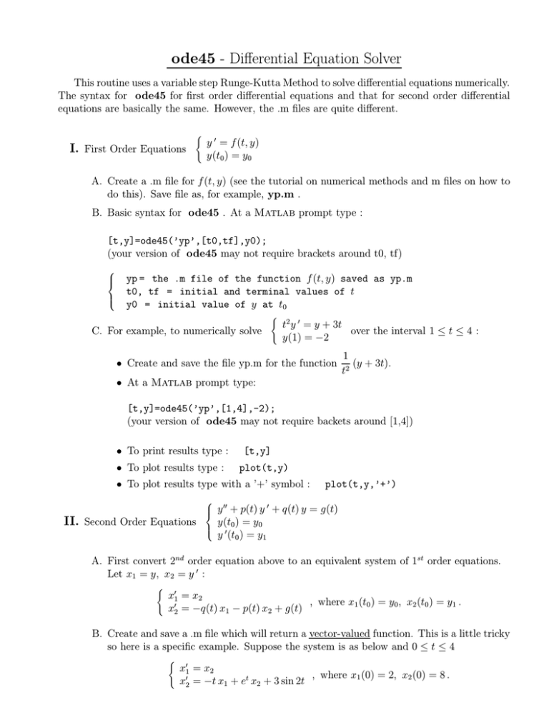
ode45 - Differential Equation Solver
This routine uses a variable step Runge-Kutta Method to solve differential equations numerically.
The syntax for ode45 for first order differential equations and that for second order differential
equations are basically the same. However, the .m files are quite different.
(
I. First Order Equations
y 0 = f (t, y)
y(t0 ) = y0
A. Create a .m file for f (t, y) (see the tutorial on numerical methods and m files on how to
do this). Save file as, for example, yp.m .
B. Basic syntax for ode45 . At a Matlab prompt type :
[t,y]=ode45(’yp’,[t0,tf],y0);
(your version of ode45 may not require brackets around t0, tf)





yp = the .m file of the function f (t, y) saved as yp.m
t0, tf = initial and terminal values of t
y0 = initial value of y at t0
(
C. For example, to numerically solve
t2 y 0 = y + 3t
over the interval 1 ≤ t ≤ 4 :
y(1) = −2
• Create and save the file yp.m for the function
• At a Matlab prompt type:
1
(y + 3t).
t2
[t,y]=ode45(’yp’,[1,4],-2);
(your version of ode45 may not require backets around [1,4])
• To print results type :
• To plot results type :
[t,y]
plot(t,y)
• To plot results type with a ’+’ symbol :
II. Second Order Equations
plot(t,y,’+’)

00
0

 y + p(t) y + q(t) y = g(t)


y(t0 ) = y0
y 0 (t0 ) = y1
A. First convert 2nd order equation above to an equivalent system of 1st order equations.
Let x1 = y, x2 = y 0 :
(
x01 = x2
, where x1 (t0 ) = y0 , x2 (t0 ) = y1 .
x02 = −q(t) x1 − p(t) x2 + g(t)
B. Create and save a .m file which will return a vector-valued function. This is a little tricky
so here is a specific example. Suppose the system is as below and 0 ≤ t ≤ 4
(
x01 = x2
, where x1 (0) = 2, x2 (0) = 8 .
x02 = −t x1 + et x2 + 3 sin 2t
• Create the following function file and save it as F.m :
function xp=F(t,x)
xp=zeros(2,1); % since output must be a column vector
xp(1)=x(2);
xp(2)=-t*x(1)+exp(t)*x(2)+3*sin(2*t); % don’t forget ; after each line
• Basic syntax for ode45 . At Matlab prompt, type :
[t,x]=ode45(’F’,[t0,tf],[x10,x20]);









F=
t0,
x10
x20
the .m file of the vector-function saved as above
tf = initial and terminal values of t
= initial value of x1 at t0 : x10 = x1 (t0 )
= initial value of x2 at t0 : x20 = x2 (t0 )
The example above becomes :[t,x]=ode45(’F’,[0,4],[2,8]);
• Since x1 (t) = y, to print out the values of the solution y for t0 ≤ t ≤ tf , type :
[t,x(:,1)]
To plot the solution on a graph t vs y, type :
plot(t,x(:,1))
(This is because the vector x has 1st component x1 = y and 2nd component x2 = y 0 .)
• To plot x1 vs x2 (phase plane) type :
plot(x(:,1),x(:,2))