1
Stationary distributions and the limit
theorem
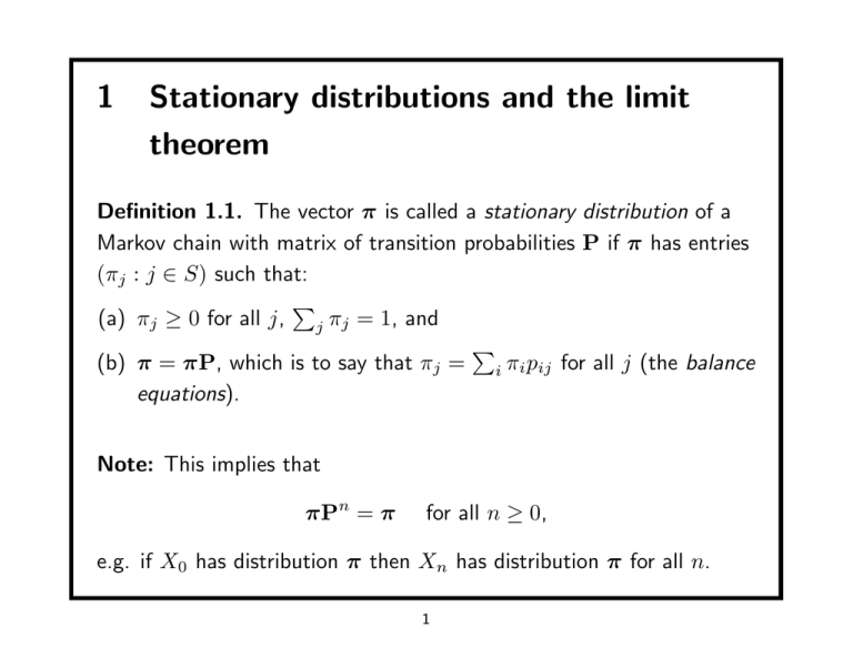
Definition 1.1. The vector π is called a stationary distribution of a
Markov chain with matrix of transition probabilities P if π has entries
(πj : j ∈ S) such that:
P
(a) πj ≥ 0 for all j, j πj = 1, and
P
(b) π = πP, which is to say that πj = i πi pij for all j (the balance
equations).
Note: This implies that
πPn = π
for all n ≥ 0,
e.g. if X0 has distribution π then Xn has distribution π for all n.
1
Proposition 1.2. An irreducible chain has a stationary distribution π
if and only if all the states are non-null persistent; in this case, π is the
unique stationary distribution and is given by πi = µ1i for each i ∈ S,
where µi is the mean recurrence time of i.
We will carry out the proof of this in several steps.
2
Fix a state k and let ρi (k) be the mean number of visits of the chain
to the state i between two successive visits to state k:
ρi (k) = E [Ni |X0 = k] ,
where
Ni =
∞
X
11{Xn = i} ∩ {Tk ≥ n}
n=1
and Tk is the time of the first return to state k. We write ρ(k) for the
P
vector (ρi (k) : i ∈ S). Clearly Tk = i∈S Ni , and hence
X
µk =
ρi (k)
i∈S
3
Lemma 1.3. For any state k of an irreducible persistent chain, the
vector ρ(k) satisfies ρi (k) < ∞ for all i, and furthermore
ρ(k) = ρ(k)P.
4
Proof. We show first that ρi (k) < ∞ when i 6= k. Observe that
ρk (k) = 1. We write
lki (n) = P {Xn = i, Tk ≥ n|X0 = k} .
Clearly fkk (m + n) ≥ lki (m)fik (n). By irreducibility of the chain,
there exists n such that fik (n) > 0. So for such a n ≥ 2
∞
X
∞
1 X
1
<∞
ρi (k) =
lki (m) ≤
fkk (m + n) ≤
f
(n)
f
(n)
ik
ik
m=1
m=1
as required.
5
Next observe that lki (1) = pki , and
X
X
lki (n) =
P (Xn = i, Xn−1 = j, Tk ≥ n|X0 = k) =
lkj (n−1)pji .
j:j6=k
j:j6=k
Summing over n ≥ 2, we obtain


X X
X

ρi (k) = pki +
lkj (n − 1)pji  = ρk (k)pki +
ρj (k)pji ,
j:j6=k
n≥2
j:j6=k
since ρk (k) = 1.
6
We have shown that for any irreducible chain, the vector ρ(k) satisfies
ρ(k) = ρ(k)P, and furthermore that the components of ρ(k) are
non-negative with sum µk . Hence, if µk < ∞, the vector π with
entries πi = ρi (k)/µk is a distribution satisfying π = πP.
Therefore, every non-null persistent irreducible chain has a stationary
distribution.
7
Proposition 1.4. For any irreducible, persistent Markov chain with
matrix of transition probabilities P, there exists a positive solution x
to the equation
x = xP,
which is unique up to a multiplicative constant. The chain is non-null
P
P
if i xi < ∞ and null if i xi = ∞.
We’ve seen all of this except for the uniqueness claim, which we
won’t establish – although it isn’t difficult.
8
Proof of Proposition (1.2) Suppose the π is a stationary distribution of
the chain. If all states are transient then pij (n) → 0 as n → ∞, for all
i and j. So
X
πj =
πi pij (n) → 0 as n → ∞
for all i and j,
i
which contradicts
P
j
πj = 1.
9
We show next that the existence of π implies that all states are
non-null and that πi = µ1i for each i. Suppose that X0 has
distribution π, so that P {X0 = i} = πi for each i. Then
πj µj = P {X0 = j}
∞
X
P {Tj ≥ n|X0 = j} =
n=1
∞
X
n=1
10
P {Tj ≥ n, X0 = j} .
However, P {Tj ≥ 1, X0 = j} = P {X0 = j}, and for n ≥ 2,
P {Tj ≥ n, X0 = j}
= P {X0 = j, Xm 6= j for 1 ≤ m ≤ n − 1}
= P {Xm 6= j for 1 ≤ m ≤ n − 1} − P {Xm 6= j for 0 ≤ m ≤ n − 1}
= P {Xm 6= j for 0 ≤ m ≤ n − 2} − P {Xm 6= j for 0 ≤ m ≤ n − 1}
by stationarity
= an−2 − an−1
where an = P {Xm 6= j for 0 ≤ m ≤ n}.
11
Sum over n to obtain
πj µj = P {X0 = j} + P {X0 6= j} − lim an = 1 − lim an .
n→∞
n→∞
However, an → P {Xm 6= j for all m} = 0 as n → ∞, by the
persistence of j. We have shown that
πj µj = 1,
so that µj = π1j < ∞ if πj > 0. To see that πj > 0 for all j, suppose
on the contrary that πj = 0 for some j.
12
Then
0 = πj =
X
πi pij (n) ≥ πi pij (n)
for all i and n,
i
yielding that πi = 0 whenever i → j. The chain is assumed irreducible,
so that πi = 0 for all i in contradiction of the fact that πi ’s sum to 1.
Hence µj < ∞ and all states of the chain are non-null. Furthermore,
we see that πj are specified uniquely as µ1j .
13
Thus, if π exists then it is unique and all the states of the chain are
non-null persistent. Conversely, if the states of the chain are non-null
persistent then the chain has a stationary distribution given by
Lemma (1.3).
14
Proposition 1.5. If i ↔ j then i is null persistent if and only if j is
null persistent.
Proof. Let C(i) be the irreducible closed equivalence class of states
which contains the non-null persistent state i. Suppose that
X0 ∈ C(i). Then Xn ∈ C(i) for all n, and Lemma (1.3) and
Proposition (1.2) combine to tell us that all the states in C(i) are
non-null.
15
Proposition 1.6. Let s ∈ S be any state of an irreducible chain. The
chain is transient if and only if there exists a non-zero solution
{yi : i 6= s}, satisfying |yi | ≤ 1 for all i, to the equations
X
yi =
pij yj ,
i 6= s.
j:j6=s
16
1.0.1
Example: Random walk with retaining barrier
A particle performs a random walk on the non-negative integers with a
retaining barrier at 0. The transition probabilities are
p0,0 = q,
pi,i+1 = p
for i ≥ 0
pi,i−1 = q
for i ≥ 1,
Let ρ = p/q.
(a) If q < p, take s = 0 to see that yi = 1 − ρ1i satisfies the equation
in Proposition (1.6), and so the chain is transient.
17
(b) Solve the equation π = πP to find that there exists a stationary
distribution, with πj = ρj (1 − ρ), if and only if q > p. Thus the
chain is non-null persistent if and only if q > p.
(c) If q = p = 21 the chain is persistent since symmetric random walk
is persistent (just reflect negative excursions of a symmetric
random walk into the positive half-line). Solve the equation
x = xP to find that xi = 1 for all i is the solution, unique up to a
P
multiplicative constant. However, i xi = ∞ so that the chain is
null by Proposition (1.4).
18
Theorem 1.7. For an irreducible aperiodic chain, we have that
pij (n) →
1
µj
as n → ∞,
for all i and j.
Proof. If the chain is transient the the result is trivial.
Suppose X is an irreducible, aperiodic, non-null, persistent Markov
chain. Construct the “coupled chain” Z = (X, Y ), as an ordered pair
X = {Xn : n ≥ 0}, Y = {Yn : n ≥ 0} of independent Markov chains,
each having state space S and transition matrix P. Then
Z = {Zn = (Xn , Yn ) : n ≥ 0} takes values in S × S, and it is easy to
check that Z is a Markov chain with transition probabilities
pij,kl = P (Zn+1 = (k, l)|Zn = (i, j))
= P (Xn+1 = k|Xn = i) P (Yn+1 = l|Yn = j)
= pik pjl
19
by independence
Since X is irreducible and aperiodic then Z is also irreducible. Since X
is non-null persistent it has a unique stationary distribution π, and it is
easy to see that Z has a stationary distribution ν = (νij : i, j ∈ S)
given by νij = πi πj ; thus Z is also non-null persistent.
20
Now suppose that X0 = i and Y0 = j, so that Z0 = (i, j). Choose any
state s ∈ S and let
T = min {n ≥ 1 : Zn = (s, s)}
denote the time that Z first hits (s, s). Note that P {T < ∞} = 1.
Starting from Z0 = (X0 , Y0 ) = (i, j)
pik (n)
= P {Xn = k}
=
P {Xn = k, T ≤ n} + P {Xn = k, T > n}
=
P {Yn = k, T ≤ n} + P {Xn = k, T > n} ,
since given T ≤ n, Xn and Yn are identically distributed. Also,
≤ P {Yn = k} + P {T > n}
= pjk (n) + P {T > n} .
21
This, and the related inequality with i and j interchanged, yields
|pik (n) − pjk (n)| ≤ P {T > n} → 0
as
n → ∞;
therefore,
pik (n) − pjk (n) → 0
as n → ∞
for all i,j and k.
Thus, if limn→∞ pik (n) exists, then it does not depend on i. To show
that it exists, write
X
πk − pjk (n) =
πi (pik (n) − pjk (n)) → 0 as n → ∞.
i
22
1.1
1.1.1
Examples
Example: The age of a renewal process
Initially an item is put into use, and when it fails it is replaced at the
beginning of the next time period by a new item. Suppose that the
lives of the items are independent and each will fail in its ith period of
use with probability Pi , i ≥ 1, where the distribution {Pi } is aperiodic
P
and i iPi < ∞. Let Xn denote the age of the item in use at time n
— that is, the number of periods (including the nth) it has been in
use.
23
Then if we let
Pi
P
λi = ∞
j=i
Pj
denote the probability that a unit that has lived for i − 1 time units
fails on the ith time unit, then {Xn , n ≥ 0} is a Markov chain with
transition probabilities given by
Pi,1 = λi = 1 − Pi,i+1 ,
i ≥ 1.
Hence the limiting probabilities are such that
π1 =
X
πi λ(i),
i
πi+1 = πi (1 − λi ),
24
i ≥ 1.
Since
P∞
j=i+1 Pj
P∞
j=i Pj
(1 − λi ) =
,
iterating yields
πi+1
=
πi (1 − λi )
=
πi−1 (1 − λi )(1 − λi−1 )
=
π1 (1 − λ1 )(1 − λ2 ) · · · (1 − λi )
∞
X
π1
Pj
=
j=i+1
=
π1 P {X ≥ i + 1} ,
where X is the life of an item.
25
Using
P∞
i=1
πi = 1 yields
1 = π1
∞
X
P {X ≥ i}
i=1
or
π1 =
1
E [X]
and hence
P {X ≥ i}
πi =
,
E [X]
i ≥ 1.
This is an example of a size-biased distribution.
26
1.1.2
Example: Poisson births
Suppose that during each time period, each member of a population
dies independently of the others with probability p, and that a
Poisson(λ) number of new members join the population each time
period. If we let Xn denote the number of members of the population
at the beginning of period n, then it is easy to see that
{Xn , n = 1, . . .} is a Markov chain.
To find the stationary distribution of this chain, suppose that X0 has a
Poisson distribution with mean α. Since each of these X0 individuals
will independently be alive at the beginning of the next period with
probability 1 − p, by the Poisson marking theorem, the number of
them that are still in the population at time 1 is a Poisson random
variable with mean α(1 − p).
27
As the number of new members that join the population at time 1 is an
independent Poisson random variable with mean λ, it thus follows that
X1 is a Poisson random variable with mean α(1 − p) + λ. Hence, if
α = α(1 − p) + λ
then the chain is stationary. By uniqueness of the stationary
distribution, we can conclude that the stationary distribution is
Poisson with mean λ/p. That is,
πj = e−λ/p (λ/p)j /j!,
28
j = 0, 1, . . .
1.1.3
Example: the Gibbs sampler
Let p(x1 , . . . , xn ) be the joint probability mass function of the random
vector (X1 , . . . , Xn ). In some cases, it may be difficult to directly
sample from such a distribution, but relatively easy to sample from the
conditional distributions of each coordinate Xi given the values of all
of the other coordinates Xj , j 6= i.
In this case, we can generate a random vector whose probability mass
function is approximately p(x1 , . . . , xn ) by constructing a Markov
chain whose stationary distribution is p as follows.
29
Let X 0 = (X10 , . . . , X10 ) be any vector for which p(X10 , . . . , Xn0 ) > 0.
First we generate a random variable whose distribution is the
conditional distribution of the first coordinate X1 given that
Xj = Xj0 , j = 2, . . . , n, and call its value X11 .
Next, generate a random variable whose distribution is the conditional
distribution of X2 given that X1 = X11 , and Xj = Xj0 , j = 3, . . . , n,
and call its value X21 .
Continue in this fashion until we have a whole new vector
X1 = (X11 , . . . , Xn1 ). Then, repeat the process, this time starting with
X1 in place of X0 , to obtain the new vector X2 , and so on. It is easy
to see that the sequence of vectors Xj , j ≥ 0 is a Markov chain. We
claim that its stationary distribution is p(x1 , . . . , xn ).
30
To verify the claim, suppose that X 0 has probability mass function
p(x1 , . . . , xn ). Then it is easy to see that at any point in this
j
, Xij−1 , . . . , Xnj−1 will be the value
algorithm the vector X1j , . . . , Xi−1
of a random variable with mass function p(x1 , . . . , xn ). For instance,
letting Xij be the random variable that takes on the value denoted by
xji then
1
0
P X1 = x1 , Xj = xj , j = 2, . . . , n
1
0
= P X1 = x1 |Xj = xj , j = 2, . . . , n
0
× P Xj = xj , j = 2, . . . , n
= P {X1 = x1 |Xj = xj , j = 2, . . . , n}
× P {Xj = xj , j = 2, . . . , n}
= p(x1 , . . . , xn ).
31
Therefore, p(x1 , . . . , xn ) is a stationary probability distribution, so
provided that the Markov chain is irreducible and aperiodic, we can
conclude that it is the limiting probability vector for the Gibbs sampler.
It also follows from the proceeding that p(x1 , . . . , xn ) would be the
limiting probability vector even if the Gibbs sampler were not
systematic in first changing the value of X1 , then X2 , and so on.,
Indeed, even if the component whose value was to be changed was
always randomly determined, then p(x1 , . . . , xn ) would remain a
stationary distribution, and would thus be the limiting probability mass
function provided that the resulting chain is aperiodic and irreducible.
32
2
Exercises
1) Each day one of n possible elements is requested; it is the ith one
Pn
with probability Pi , i ≥ 1, i=1 Pi = 1. These elements are at all
times arranged in an ordered list that is revised as follows: the element
selected is moved to the front of the list, and the relative positions of
all other elements remain unchanged. Define the state at any time to
be the ordering of the list at that time.
(a) Argue that the above is Markov chain.
(b) For any state (i1 , . . . , in ) (which is a permutation of (1, 2, . . . , n))
let π(i1 , . . . , in ) denote the limiting probability. Argue that
π(i1 , . . . , in ) = Pi1
Pin−1
Pi 2
···
.
1 − Pi 1
1 − Pi1 − · · · − Pin−2
33
2) Let {Xn , n ≥ 0} be a Markov chain with stationary probabilities πj ,
j ≥ 0. Suppose that X0 = 0 and define
T = min{n > 0 : Xn = 0}.
Let Yj = XT −j , j = 0, 1, . . . , T . Show that {Yj , j = 0, . . . , T } is
distributed as the states visited by a Markov chain (the “reversed”
Markov chain) with transition probabilities Pij∗ = πj Pji /πi started in
state 0 and watched until it returns to 0.
34
3) Consider a finite Markov chain on the state space {0, 1, 2, . . . , N }
with transition probability matrix P = (Pij )N
i,j=0 , and divide the state
space into the three classes {0}, {1, 2, . . . , N − 1} and {N }. Let 0
and N be absorbing states, both accessible from all states in
1, . . . , N − 1, and let {1, 2, . . . , N − 1} be a transient class.
Let k be a transient state. Define an auxiliary process (the “return
process”) with transition matrix Pe by altering the first and last row of
P so that Pe0k = PeN k = 1 and leave the other rows unchanged.
The return process is clearly irreducible. Prove that the expected time
until absorption µk with initial state k in the original process equals
1/(π0 + πN ) − 1 where π0 + πN is the stationary probability of being
in state 0 or N for the return process.
Hint: use the relation between stationary probabilities and expected
recurrence times to states.
35
3
Reversibility
Suppose that {Xn : 0 ≤ n ≤ N } is an irreducible, non-null, persistent
Markov chain, with transition matrix P and stationary distribution π.
Suppose further that Xn has distribution π for every n. Define the
’reversed chain’ Y by Yn = XN −n for 0 ≤ n ≤ N .
36
Proposition 3.1. The sequence Y is a Markov chain with
P{Y0 = i} = πi and
P {Yn+1
πj
= j|Yn = i} =
pji .
πi
We call the chain Y the time reversal of chain X, and we say that X
is reversible if X and Y have the same transition probabilities.
37
Proof. The crucial step is the stationarity of X:
P {Yn+1 = in+1 |Yn = in , Yn−1 = in−1 , . . . , Y0 = i0 }
P {Yk = ik , 0 ≤ k ≤ n + 1}
=
P {Yk = ik , 0 ≤ k ≤ n}
P {XN −n−1 = in+1 , XN −n = in , . . . , XN = i0 }
=
P {XN −n = in , . . . , XN = i0 }
πi pi ,i pi ,i
. . . pi1 ,i0
= n+1 n+1 n n n−1
πin pin ,in−1 . . . pi1 ,i0
πin+1 pin+1 ,in
=
.
πin
38
Let X = {Xn : 0 ≤ n ≤ N } be an irreducible Markov chain such that
Xn has the stationary distribution π for all n. The chain is called
reversible if the transition matrices of X and its time-reversal Y are
the same, which is to say that
πi pij = πj pji
for all i,j.
These equations are called the detailed balance equations.
39
Proposition 3.2. Let P be the transition matrix of an irreducible
chain X, and suppose that there exists a distribution π such that
πi pij = πj pji for all i,j ∈ S. Then π is a stationary distribution of the
chain.
40
Proof. Suppose that π satisfies the conditions above. Then
X
X
X
πi pij =
πj pji = πj
pji = πj
i
i
i
and so π = πP, whence π is stationary.
41
3.1
3.1.1
Reversible Examples
Example: Ehrenfest model of diffusion
Two containers A and B are placed adjacent to each other and gas is
allowed to pass through a small aperture joining them. A total of m
gas molecules is distributed between the containers. We assume that
at each epoch of time one molecule, picked uniformly at random from
the m available, passes through this aperture. Let Xn be the number
of molecules in container A after n units of time has passed. Clearly
{Xn } is a Markov chain with transition matrix
pi,i+1
i
=1− ,
m
pi,i−1
42
i
=
m
if 0 ≤ i ≤ m.
Rather than solve the equation π = πP to find the stationary
distribution, we look for solutions of the detailed balance equations
πi pij = πj pji
.
This is solved by πi =
distribution.
m
i
( 12 )m , which is therefore the stationary
43
3.1.2
Example: the Metropolis algorithm
Pm
Let aj ,j = 1, . . . , m be positive numbers and let A = j=1 aj .
Suppose that m is large and that A is difficult to compute, and
suppose we ideally want to simulate the values of a sequence of
independent random variables whose probabilities are pj = aj /A, for
j = 1, . . . , m.
Similar to the Gibbs sampler, one way of simulating a sequence of
random variables whose distributions converge to {pj , j = 1, . . . , m} is
to find a Markov chain that is both easy to simulate and whose
limiting probabilities are the pj . The Metropolis algorithm provides an
approach for accomplishing this task.
44
Let Q be any irreducible transition probability matrix on the integers
1, 2, . . . , n such that qij = qji for all i and j. Now define a Markov
chain {Xn , n ≥ 0} as follows. If Xn = i, then generate a random
variable that is equal to j with probability qij , i, j = 1, . . . , m. If this
random variable takes on the value j, then set Xn+1 equal to j with
probability min{1, aj /ai }, and set it equal to i otherwise.
That is, the transition probabilities of {Xn , n ≥ 0} are

q min(1, a /a )
ij
j
i
Pij =
qii + P qij {1 − min(1, aj /ai )}
j6=i
45
if j 6= i,
if j = i.
We will now show that the stationary distribution of this Markov chain
is given by the pj .
We will first show that the chain is reversible with stationary
probabilities pj , j = 1, . . . , m by showing that
pi Pij = pj Pji .
To show this, we must show that
pi qij min(1, ai /aj ) = pj qji min(1, aj /ai ).
Now, qij = qji and aj /ai = pj /pi and so we must verify that
pi min(1, pj /pi ) = pj min(1, pi /pj ).
This is immediate since both sides of the equation are equal to
min(pi , pj ).
46
That these stationary probabilities are also limiting probabilities follows
from the fact that since Q is an irreducible transition probability
matrix, {Xn } will also be irreducible, and as Pii > 0 for some i
(except in the trivial case where pi ≡ 1/n), it is also aperiodic.
By choosing a transition probability matrix Q that is easy to simulate
– that is, for each i it is easy to generate the value of a random
variable that is equal to j with probability qij – we can use the
preceding to generate a Markov chain whose limiting probabilities are
aj /A, without computing A.
47
3.1.3
Example: Random walk on a graph
Consider a graph having a positive number wij associated with each
edge (i, j), and suppose that a particle moves from vertex to vertex in
the following manner:
If the particle is at vertex i then it will move to vertex j with
probability proportional to the outgoing edge weights:
Pij = wij /
X
wij
j
where wij is 0 if (i, j) is not an edge of the graph. The Markov chain
describing the sequence of vertices visited by the particle is called a
random walk on an edge weighted graph.
48
Proposition 3.3. Consider a random walk on an edge weighted graph
with a finite number of vertices. If this Markov chain is irreducible,
then in steady state it is time reversible with stationary probabilities
given by
P
i wij
P
P
.
πi =
w
j
i ij
Proof. The time reversible equations
πi Pij = πj Pji
reduce to
πw
π w
Pi ij = Pj ji
k wik
k wjk
49
or, equivalently, since wij = wji
πj
πi
=P
k wik
k wjk
P
implying that
πi = c
X
k
Since
P
πi = 1, we are done.
50
wik .
4
Exercises
1) Consider a time-reversible Markov chain on the state space
{0, 1, 2, . . .} with transition probabilities Pij and limiting probabilities
πi . Suppose we truncate the chain to the states {0, 1, . . . , M } by
defining the transition probabilities

P


Pij + k>M Pik , 0 ≤ i ≤ M, j = i
P ij = Pij ,
0 ≤ i 6= j ≤ M



0,
otherwise.
Show that the truncated chain is also time reversible and has limiting
probabilities given by
πi
π i = PM
i=0
51
πi
.
2) Suppose M balls are initially distributed among m urns. At each
stage one of the balls is selected at random, taken from whichever urn
it is in, and placed, again at random, in one of the other m − 1 urns.
Consider the Markov chain whose state at any time is the vector
(n1 , . . . , nm ), where ni denotes the number of balls in urn i. Guess at
the limiting probabilities for this Markov chain and verify your guess,
showing at the same time that the Markov chain is time reversible.
52