GMT TECHNICAL REFERENCE & COOKBOOK
5–1
1
5. GMT Projections
GMT programs that read position data will need to know how to convert the input
coordinates to positions on the map. This is achieved by selecting one of several
projections. The purpose of this section is to summarize the properties of map
projections available in GMT, what parameters define them, and demonstrate how they
are used to create simple basemaps. We will mostly be using the pscoast command and
occasionally psxy. (Our illustrations may differ from yours because of different settings
in our .gmtdefaults file.) Note that while we will refer to lengths and scales in inches,
you may want to use cm as unit instead (see gmtdefaults man page).
5.1 Non-map Projections
5.1.1 Linear Projection (–Jx or –JX)
The linear projection comes in three flavors: linear, log10, and power. The projection
for the y-axis can be set independently from the x-axis. We will show examples of all
three by first creating dummy data sets using sample1d and nawk (or awk):
sample1d -I1 -L << END | nawk '{print $1, sqrt ($1)}' > sqrt.d
0 0
100
0
END
sample1d -I10 -L << END | nawk '{print $1, sqrt ($1)}' > sqrt.d10
0 0
100
0
END
The projection is defined by stating
• scale in inches/unit (–Jx) or axis length in inches (–JX)
If the y-scale or y-axis length is different from that of the x-axis (which is most often the
case), separate the two scales (or lengths) by a slash, e.g., –Jx0.1/0.5 or –JX8/5.
Linear projection
Selection of this transformation will result in a linear scaling of the input coordinates.
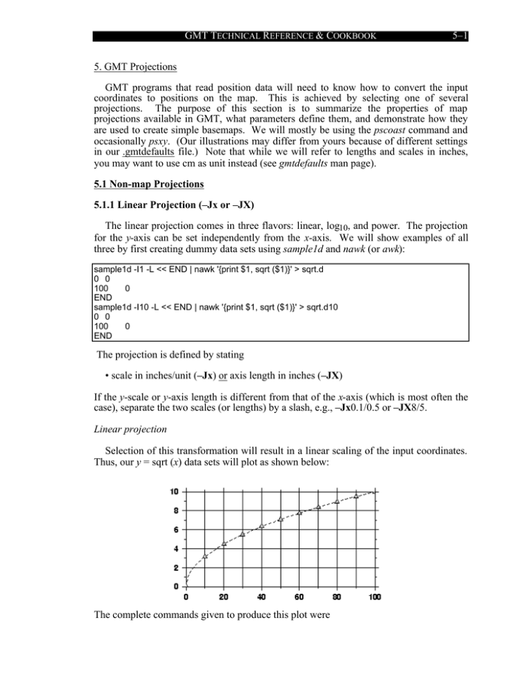
Thus, our y = sqrt (x) data sets will plot as shown below:
The complete commands given to produce this plot were
GMT TECHNICAL REFERENCE & COOKBOOK
5–2
2
psxy -R0/100/0/10 -JX4/2 -Ba20f10g10/a2f1g2WSne -W5t15_15:0 -P -K -X0.5 -Y0.5 sqrt.d >
linear.ps
psxy -R -JX -St0.1 -G200 -W -O sqrt.d10 >> linear.ps
Normally, the user's x-values will increase to the right and the y-values will increase
upwards. It should be noted that in many situations it is desirable to have the direction of
positive coordinates be reversed. For example, when plotting depth on the y-axis it
makes more sense to have the positive direction downwards. All that is required to
reverse the sense of positive direction is to supply a negative scale (or axis length).
Logarithmic projection
The log10 transformation is selected by appending an l (lower case L) immediately
following the scale (or axis length) value. Hence, to produce a plot in which the x-axis is
logarithmic (the y-axis remains linear), try
psxy -R1/100/0/10 -Jx2l/0.2 -B2g3/a2f1g2WSne -W5t5_5:0 -P -K -X0.5 -Y0.5 -H sqrt.d > log.ps
psxy -R -Jx -Ss0.1 -G0 -W -O -H sqrt.d10 >> log.ps
Note that if x- and y-scaling are different and a log10-log10 plot is desired, the l must be
appended twice: Once after the x-scale (before the /) and once after the y-scale.
Power projection
This projection allows us to display xa versus yb. While a and b can be any value, we
will select a = 0.5 and b = 1 which means we will plot y versus x. We indicate this
scaling by appending a p (lower case P) followed by the desired exponent, in our case
0.5. Since b = 1 we do not need to specify p1 since it is identical to the linear scaling.
Thus our command becomes
psxy -R0/100/0/10 -Jx0.4p0.5/0.2 -Ba1p/a2f1WSne -W5 -P -K -X0.5 -Y0.5 sqrt.d > pow.ps
psxy -R -Jx -Sc0.1 -G255 -W -O sqrt.d10 >> pow.ps
GMT TECHNICAL REFERENCE & COOKBOOK
5–3
3
While these linear projections are primarily designed for generic x-y data, it is
sometimes necessary to plot geographical data in a linear projection. This poses a
problem since longitudes have a 360 degree periodicity. GMT therefore needs to be
informed that it has been given geographical data although a linear projection has been
chosen. We do so by appending a d (for degrees) to the –Jx (or –JX) option. As an
example, we want to plot a crude world map centered on 125˚E. Our command will be
gmtset GRID_CROSS_SIZE 0.1 BASEMAP_TYPE FANCY DEGREE_FORMAT 3
pscoast -R-55/305/-90/90 -Jx0.014d -B60g30f15/30g30f15WSen -Dc -G200 -W1 -P -X0.5 -Y0.5 >
degree.ps
with the result reproduced below.
GMT TECHNICAL REFERENCE & COOKBOOK
5–4
4
5.1.2 Linear Projection with Polar ( , r) Coordinates (–Jp or –JP)
In many applications the data is better described in polar or cylindrical ( , r)
coordinates rather than the usual Cartesian coordinates (x, y). The relationship between
the Cartesian and polar coordinates are described by x = r·cos , y = r·sin . The polar
transformation is simply defined by providing
• scale in inches/unit (–Jp) or full width of plot in inches (–JP).
As an example of this projection we will create a gridded data set in polar coordinates
z( , r) = r2 ·cos(4 ) using grdmath, a "Reverse Polish Notation" (RPN) calculator that
operates on or creates grdfiles. We could also create the data with xyz2grd and the UNIX
tool nawk: (0.06981317 = 4 · (360˚/2π)); its command line is commented out in the
script below.
#nawk 'BEGIN {for (theta = 0; theta <= 360; theta += 6) {for (r = 2.0; r <= 4.01; r += 0.1) print
theta, r, cos (0.06981317 * theta) * r * r}}' /dev/null | xyz2grd -R0/360/2/4 -I6/0.1 -Gtest.grd
grdmath -R0/360/2/4 -I6/0.1 X 4 MUL PI MUL 180 DIV COS Y 2 POW MUL = test.grd
grdcontour test.grd -JP4 -B30Ns -P -C2 -S4 -X0.5 -Y0.5 > donut.ps
We used grdcontour to make a contour map of this data. Because the data file only
contains values with 2 ≤ r ≤ 4, a donut shaped plot appears below.