Supply and Demand
advertisement

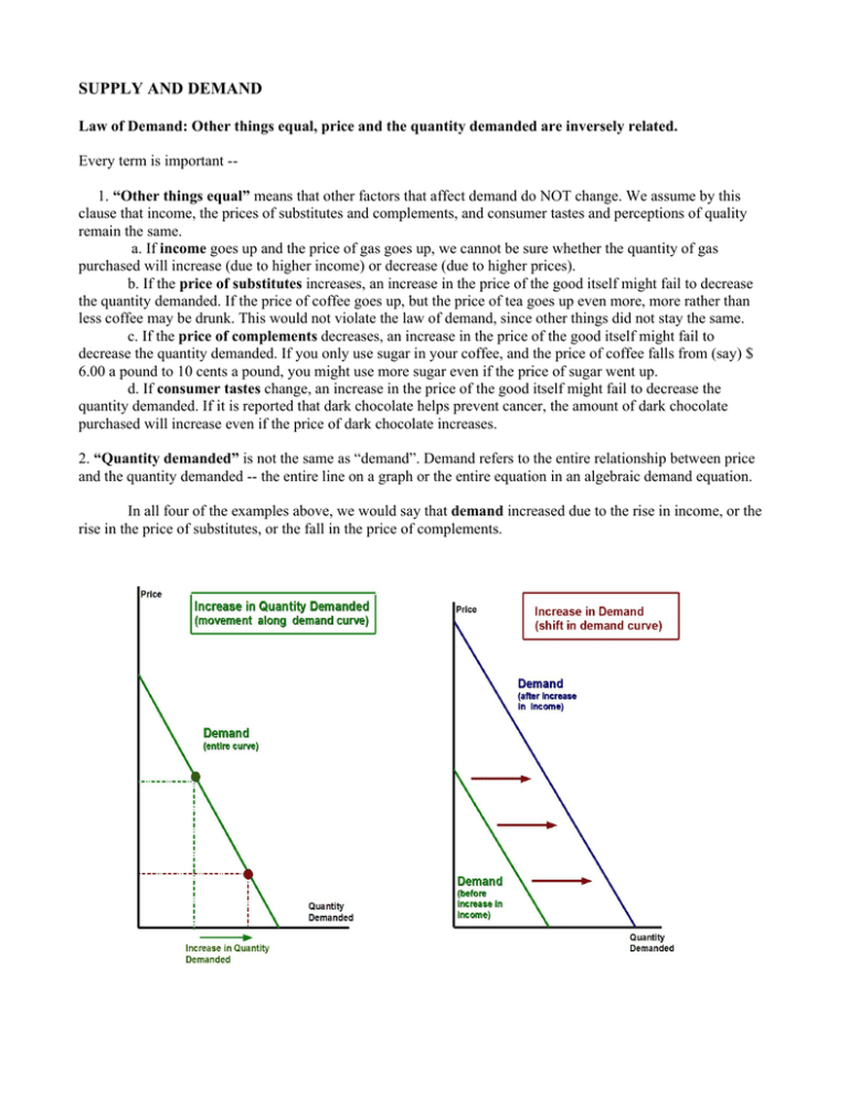
SUPPLY AND DEMAND Law of Demand: Other things equal, price and the quantity demanded are inversely related. Every term is important -1. “Other things equal” means that other factors that affect demand do NOT change. We assume by this clause that income, the prices of substitutes and complements, and consumer tastes and perceptions of quality remain the same. a. If income goes up and the price of gas goes up, we cannot be sure whether the quantity of gas purchased will increase (due to higher income) or decrease (due to higher prices). b. If the price of substitutes increases, an increase in the price of the good itself might fail to decrease the quantity demanded. If the price of coffee goes up, but the price of tea goes up even more, more rather than less coffee may be drunk. This would not violate the law of demand, since other things did not stay the same. c. If the price of complements decreases, an increase in the price of the good itself might fail to decrease the quantity demanded. If you only use sugar in your coffee, and the price of coffee falls from (say) $ 6.00 a pound to 10 cents a pound, you might use more sugar even if the price of sugar went up. d. If consumer tastes change, an increase in the price of the good itself might fail to decrease the quantity demanded. If it is reported that dark chocolate helps prevent cancer, the amount of dark chocolate purchased will increase even if the price of dark chocolate increases. 2. “Quantity demanded” is not the same as “demand”. Demand refers to the entire relationship between price and the quantity demanded -- the entire line on a graph or the entire equation in an algebraic demand equation. In all four of the examples above, we would say that demand increased due to the rise in income, or the rise in the price of substitutes, or the fall in the price of complements. What does the demand curve show? 1. The reservation price or the maximum price that some consumer would be willing (if necessary) to pay for a given amount of the good. Note that “willing” does not mean “willing and eager” -- the consumer will be happy if he can obtain the good for less. If the consumer pays less than he is willing to pay, he enjoys a consumer surplus equal to the difference between his willingness to pay and the market price. [Imagine that people are lined up along the demand curve, with the person willing to pay the greatest price at the top (the Yaxis intercept) of the demand curve, and one who doesn't value the good at all at the bottom (the X-axis intercept) of the demand curve.] 2. The maximum amount of a good which consumers would be willing to buy at a given price. Algebra of the demand curve Since the demand curve shows a negative relation between quantity demanded and price, the curve representing it must slope downwards. If the demand equation is linear, it will be of the form: P = a - b Qd where a is the intercept along the Y-axis (the highest price anyone would pay) and b is the slope of the equation. A numerical example can be easily translated into a graph: Check your understanding by: a. Plotting the curve P = 800 - 3 Qd [Hint: since slopes are the same, the lines will be parallel] b. Letting the Y-intercept be 500 and the X-intercept be 400 and calculating the equation. [Hint: slope = rise/run, and note that the slope will be negative and greater than 1] SUPPLY Law of supply: Other things equal, price and the quantity supplied are (almost always) positively related. What does the supply curve show? It shows the lowest price at which producers are willing to sell. The lowest price at which producers would be willing to sell is the cost of production, or more specifically the marginal cost of production -- the cost of producing another unit of the good. Of course, they would be happier if the price were higher than the cost. Almost always: Normally (but not always) the marginal cost of production does rise with output, because producers face different cost conditions. In Saudi Arabia, it costs $10 or less to produce a barrel of oil; in Iran, it costs $15; in Nigeria, $20; from North Sea oil rigs, $25. The price of oil must rise to $25 or more a barrel in order to make it profitable to drill in the North Sea. The upward slope of the supply curve reflects rising marginal costs; if marginal costs do not rise, the supply curve would be horizontal. You will sometimes see flat supply curves to simplify the graphs in the discussion of monopoly in microeconomics, and to illustrate the possibility of expanding national output (GDP) at low additional cost in macroeconomic discussions of recession. You may also see vertical supply curves: the supply of Rembrandt paintings is fixed, so an increase in price will not increase the quantity of Rembrandt paintings supplied. In macroeconomics, if we have full employment, we cannot produce any more just because prices go up (there is no one to produce them), so the aggregate supply curve will be vertical. Other things equal: if “other things” that affect overall cost conditions do change, the supply curve will shift. If costs become greater (higher wages, bad weather for crops), producers will want a higher price in order to produce the same amount of the good; if they cannot get the higher price, some (the high cost producers) will go out of business. Note that the reaction to a change in costs may differ by industry: if oil prices go up, more oil will be produced (a movement along the oil industry supply curve), but there will be an upward shift in the supply curve of oil-using industries . If improvements in technology make it possible to produce goods at a lower marginal cost of production, the supply curve will shift downward. If they had to, producers would be willing to sell the same quantity of goods for a lower price. Of course, they are not eager to, and will only cut prices if the interaction of supply and demand forces them to. Thinking of supply shifts as a change in the cost of production, and connecting the shift with the desire of producers for higher prices (or their willingness to accept lower prices) is the best way of understanding what is happening. You must also however realize that when costs of production rise, we can also speak of a decrease in supply. This can be confusing at first, since the supply curve shifts upward on the graph. Note in the graphs on the next page show that if the supply curve shifts upward, a smaller quantity will be supplied at any given price. The only significant change between the two graphs is whether the arrows showing the shift are drawn upwards or from right to left. The same shift occurs whether you think of it as: a. higher costs of production mean that producers require higher prices to produce the same output. b. if prices stay the same, a smaller quantity will be supplied. Both supply and demand curves are best used for studying the economics of the short run. In the long run, a. demand curves will become flatter as consumers adjust to big changes in the markets. Drivers don't sell their SUV next week when gas prices go up sharply, but if they stay up their next vehicle may well be a small car. b. supply curves may change even more drastically: Producers can build more factories, and this reduces the marginal cost of additional output, so flattening the slope of the supply curve. (The definition of the long run is the amount of time needed to increase factors of production other than labor or raw materials; for manufacturing, this means the amount of time to build a new factory) New larger scale factories may enjoy economies of scale, which means the supply curve may in the longer run appear to slope downward. Both (a) and (b) mean that supply and demand graphs are less useful (or at least more messy) when considering long run changes. Algebra of the supply curve Since the demand curve shows a positive relation between quantity supplied and price, the graph of the equation representing it must slope upwards. If the supply equation is linear, it will be of the form: P = a + b Qs where a is the intercept along the Y-axis (the lowest price anyone would sell for) and b is the slope of the line. A numerical example can be easily translated into a graph: Note that: -- the lowest price anyone would sell for is $ 50 -- in order to supply 100 units of the good, the price must be at a minimum $ 250. To test your understanding, try graphing the supply equations: -- P = 100 + 2 Qs (same slope, different Y-axis intercept) -- P = 50 + 3 Qs (same Y-axis intercept, different and steeper slope) and calculate the price necessary for producers to supply 100 units of the good. In fact, calculating this price will be necessary to get an accurate representation of the supply curves.


