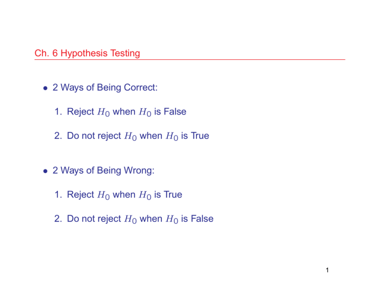
Ch. 6 Hypothesis Testing
• 2 Ways of Being Correct:
1. Reject H0 when H0 is False
2. Do not reject H0 when H0 is True
• 2 Ways of Being Wrong:
1. Reject H0 when H0 is True
2. Do not reject H0 when H0 is False
1
Type I Error and Level of Significance
• A False Alarm. E.g., In quality control, a manufacturing process is
monitored; it may be in control or out of control. If it is judged out of
control when really in control, this is a Type I error.
• α = level of significance
α = P (Type I Error)
This value is under the control of the experimenter, e.g. .05, .01, etc
2
Type II Error and Power
• A Missed Signal. E.g., a manufacturing process is judged to be in
control when really out of control.
• β = 1 - power
β = P (Type II Error)
Note that β is often a function of a parameter, since the alternative
hypothesis is not simple like the null hypothesis.
3
Type II Error and Power
• Example. Single-Sample Acceptance Sampling Plans
A simple random sample is selected from a lot for inspection.
◦ n = sample size.
◦ c = acceptance number.
◦ The number of defectives in the sample is denoted by D.
◦ If D > c, then the lot is rejected.
◦ Ideally, only acceptable lots would be accepted, and only
unacceptable lots would be rejected.
4
Acceptance Sampling (cont’d)
• An unacceptable lot is defined as one whose proportion defective is
greater than p0.
◦ probability of accepting the lot:
.
β(p) = P (D ≤ c) =
c
X
!
n j
p (1 − p)n−j
j=0 j
◦ p = true proportion nonconforming.
• For p > p0, β(p) gives the probability of committing a Type II error.
• Power = 1 − β(p)
• α = 1 − β(p0).
5
Acceptance Sampling (cont’d)
• Suppose an unacceptable lot is defined as one with more than 2%
defective, n = 50 and c = 1.
• Find the significance level α for the associated hypothesis test.
• Find the probability of Type II Error if the true proportion defective is
3%. What is the power of the test for such a lot?
6
Control Charts
• Measurements from an in control manufacturing process should be
independent and identically distributed random variables with mean
µ0 and variance σ 2.
• Periodically, samples of size n are taken from a process, and the
sample mean is computed. The sample mean should lie within
σ
µ0 ± 3 √
n
most of the time.
• If the sample mean lands outside the above control limits, then the
process is said to be out of control.
• H0 : process is in control
• HA : process is out of control
7
Control Charts (cont’d)
• α = P (Type I Error) =
1−P
σ
σ
µ0 − 3 √ < X̄ < µ0 + 3 √
n
n
!
= 1 − P (−3 < Z < 3) = 1 − .9973 = .0027
[Z is standard normal]
• Find the probability of Type II Error for the case where the mean has
shifted upwards by .2σ (assume n = 9).
•
β(µ0 + .2σ) = P
σ
σ
µ0 − 3 √ < X̄ < µ0 + 3 √
n
n
!
= P (−3.6 < Z < 2.4) = .9916
8
• Find P (Type II Error) if the mean has shifted upwards by .8σ.
β(µ0 + .8σ) = P (−5.4 < Z < .6) = .7257