NCSS Statistical Software
NCSS.com
Chapter 445
Hierarchical
Clustering /
Dendrograms
Introduction
The agglomerative hierarchical clustering algorithms available in this program module build a cluster hierarchy
that is commonly displayed as a tree diagram called a dendrogram. They begin with each object in a separate
cluster. At each step, the two clusters that are most similar are joined into a single new cluster. Once fused,
objects are never separated. The eight methods that are available represent eight methods of defining the
similarity between clusters.
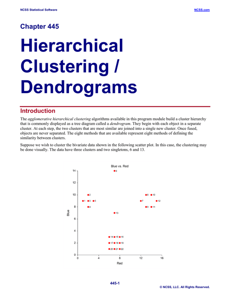
Suppose we wish to cluster the bivariate data shown in the following scatter plot. In this case, the clustering may
be done visually. The data have three clusters and two singletons, 6 and 13.
445-1
© NCSS, LLC. All Rights Reserved.
NCSS Statistical Software
NCSS.com
Hierarchical Clustering / Dendrograms
Following is a dendrogram of the results of running these data through the Group Average clustering algorithm.
Dendrogram
Row
12
11
9
10
8
7
22
19
16
21
20
18
17
15
14
13
6
5
4
2
3
1
8.00
6.00
4.00
Dissimilarity
2.00
0.00
The horizontal axis of the dendrogram represents the distance or dissimilarity between clusters. The vertical axis
represents the objects and clusters. The dendrogram is fairly simple to interpret. Remember that our main interest
is in similarity and clustering. Each joining (fusion) of two clusters is represented on the graph by the splitting of
a horizontal line into two horizontal lines. The horizontal position of the split, shown by the short vertical bar,
gives the distance (dissimilarity) between the two clusters.
Looking at this dendrogram, you can see the three clusters as three branches that occur at about the same
horizontal distance. The two outliers, 6 and 13, are fused in rather arbitrarily at much higher distances. This is the
interpretation.
In this example we can compare our interpretation with an actual plot of the data. Unfortunately, this usually will
not be possible because our data will consist of more than two variables.
Dissimilarities
The first task is to form the distances (dissimilarities) between individual objects. This is described in the Medoid
Clustering chapter and will not be repeated here.
Hierarchical Algorithms
The algorithm used by all eight of the clustering methods is outlined as follows. Let the distance between clusters
i and j be represented as d ij and let cluster i contain ni objects. Let D represent the set of all remaining d ij .
Suppose there are N objects to cluster.
1. Find the smallest element d ij remaining in D.
2. Merge clusters i and j into a single new cluster, k.
3. Calculate a new set of distances d km using the following distance formula.
d km = α i d im + α j d jm + β d ij + γ d im − d jm
445-2
© NCSS, LLC. All Rights Reserved.
NCSS Statistical Software
NCSS.com
Hierarchical Clustering / Dendrograms
Here m represents any cluster other than k. These new distances replace d im and d jm in D. Also let
n k = ni + n j .
Note that the eight algorithms available represent eight choices for α i , α j , β , and γ .
4. Repeat steps 1 - 3 until D contains a single group made up off all objects. This will require N-1 iterations.
We will now give brief comments about each of the eight techniques.
Single Linkage
Also known as nearest neighbor clustering, this is one of the oldest and most famous of the hierarchical
techniques. The distance between two groups is defined as the distance between their two closest members. It
often yields clusters in which individuals are added sequentially to a single group.
The coefficients of the distance equation are α i = α j = 0.5, β = 0, γ = −0.5.
Complete Linkage
Also known as furthest neighbor or maximum method, this method defines the distance between two groups as
the distance between their two farthest-apart members. This method usually yields clusters that are well separated
and compact.
The coefficients of the distance equation are α i = α j = 0.5, β = 0, γ = 0.5.
Simple Average
Also called the weighted pair-group method, this algorithm defines the distance between groups as the average
distance between each of the members, weighted so that the two groups have an equal influence on the final
result.
The coefficients of the distance equation are α i = α j = 0.5, β = 0, γ = 0.
Centroid
Also referred to as the unweighted pair-group centroid method, this method defines the distance between two
groups as the distance between their centroids (center of gravity or vector average). The method should only be
used with Euclidean distances.
The coefficients of the distance equation are α i =
nj
ni
,α j =
, β = −α iα j , γ = 0.
nk
nk
Backward links may occur with this method. These are recognizable when the dendrogram no longer exhibits its
simple tree-like structure in which each fusion results in a new cluster that is at a higher distance level (moves
from right to left). With backward links, fusions can take place that result in clusters at a lower distance level
(move from left to right). The dendrogram is difficult to interpret in this case.
Median
Also called the weighted pair-group centroid method, this defines the distance between two groups as the
weighted distance between their centroids, the weight being proportional to the number of individuals in each
group. Backward links (see discussion under Centroid) may occur with this method. The method should only be
used with Euclidean distances.
The coefficients of the distance equation are α i = α j = 0.5, β = −0.25, γ = 0.
445-3
© NCSS, LLC. All Rights Reserved.
NCSS Statistical Software
NCSS.com
Hierarchical Clustering / Dendrograms
Group Average
Also called the unweighted pair-group method, this is perhaps the most widely used of all the hierarchical cluster
techniques. The distance between two groups is defined as the average distance between each of their members.
The coefficients of the distance equation are α i =
nj
ni
,α j =
, β = 0, γ = 0.
nk
nk
Ward’s Minimum Variance
With this method, groups are formed so that the pooled within-group sum of squares is minimized. That is, at
each step, the two clusters are fused which result in the least increase in the pooled within-group sum of squares.
The coefficients of the distance equation are α i =
n j + nm
− nm
ni + n m
, γ = 0.
,α j =
,β =
nk + nm
nk + nm
nk + nm
Flexible Strategy
Lance and Williams (1967) suggested that a continuum could be made between single and complete linkage. The
program lets you try various settings of these parameters which do not conform to the constraints suggested by
Lance and Williams.
The coefficients of the distance equation should conform to the following constraints
α i = 1 − β − α j , α j = 1 − β − α i , − 1 ≤ β ≤ 1, γ = 0.
One interesting exercise is to vary these values, trying to find the set that maximizes the cophenetic correlation
coefficient.
Goodness-of-Fit
Given the large number of techniques, it is often difficult to decide which is best. One criterion that has become
popular is to use the result that has largest cophenetic correlation coefficient. This is the correlation between the
original distances and those that result from the cluster configuration. Values above 0.75 are felt to be good. The
Group Average method appears to produce high values of this statistic. This may be one reason that it is so
popular.
A second measure of goodness of fit called delta is described in Mather (1976). These statistics measure degree of
distortion rather than degree of resemblance (as with the cophenetic correlation). The two delta coefficients are
given by
 N

* 1/ A
 | d jk - d jk | 
 j<k

∆A = 
* 1/ A 
(
)
 j<k d jk



∑
A
∑
where A is either 0.5 or 1 and d ij* is the distance obtained from the cluster configuration. Values close to zero are
desirable.
Mather (1976) suggests that the Group Average method is the safest to use as an exploratory method, although he
goes on to suggest that several methods should be tried and the one with the largest cophenetic correlation be
selected for further investigation.
445-4
© NCSS, LLC. All Rights Reserved.
NCSS Statistical Software
NCSS.com
Hierarchical Clustering / Dendrograms
Number of Clusters
These techniques do not let you explicitly set the number of clusters. Instead, you pick a distance value that will
yield an appropriate number of clusters. This will be discussed further when we discuss the Dendrogram and the
Linkage report.
Limitations and Criticisms
We have attempted problems with up to 1,000 objects. Running times will vary with computer speed, with larger
problems running several hours. Problems with 100 objects or less should run in a few seconds.
Hierarchical clustering methods are popular because they are relatively simple to understand and implement.
However, this simplicity yields one of their strongest criticisms. Once two objects are joined, they can never be
separated. As Kaufman (1990) complains, “once the damage is done, it can never be repaired.”
Data Structure
The data are entered in the standard columnar format in which each column represents a single variable.
The data given in the following table contain information on twelve superstars in basketball. The stats are on a per
game basis for games played through the 1989 season.
BBall dataset (subset)
Player
Jabbar K.A.
Barry R
Baylor E
Bird L
Chamberlain W
Cousy B
Erving J
Height
86.0
79.0
77.0
81.0
85.0
72.5
78.5
FgPct
55.9
44.9
43.1
50.3
54.0
37.5
50.6
Points
24.6
23.2
27.4
25
30.1
18.4
24.2
Rebounds
11.2
6.7
13.5
10.2
22.9
5.2
8.5
Missing Values
When an observation has missing values, appropriate adjustments are made so that the average dissimilarity
across all variables with non-missing data is computed. Hence, rows with missing values are not omitted unless
all variables have missing values. Note that the distances require that at least one variable have non-missing
values for each pair of rows.
445-5
© NCSS, LLC. All Rights Reserved.
NCSS Statistical Software
NCSS.com
Hierarchical Clustering / Dendrograms
Procedure Options
This section describes the options available in this procedure.
Variables Tab
This panel specifies the variables used in the analysis.
Variables
Interval Variables
Designates interval-type variables (if any) or the columns of the matrix if distance or correlation matrix input was
selected. Interval variables are continuous measurements that may be either positive or negative and follow a
linear scale. Examples include height, weight, age, price, temperature, and time.
In general, an interval should keep the same importance throughout the scale. For example, the length of time
between 1905 and 1925 is the same as the length of time between 1995 and 2015.
Note that a nonlinear transformation of an interval variable is probably not an interval variable. For example, the
logarithm of height is not an interval variable since the value of an interval along the scale changes depending
upon where you are on the scale.
Ordinal Variables
Specifies the ordinal-type variables (if any). Ordinal variables are measurements that may be ordered according to
magnitude. For example, a survey question may require you to pick one of five possible choices: strongly disagree
(5), disagree (4), neutral (3), agree (2), or strongly agree (1). Interval variables are ordinal, but ordinal variables
are not necessarily interval.
The original values of ordinal variables are replaced by their ranks. These ranks are then analyzed as if they were
interval variables.
Symmetric-Binary Variables
Specifies the symmetric binary-type variables (if any). Symmetric binary variables have two possible outcomes,
each of which carry the same information and weight. Examples include gender, marital status, or membership in
a particular group. Usually, they are coded as 1 for yes or 0 for no, although this is not necessary.
These variables are analyzed using the number of matches between two individuals.
Ratio Variables
Specifies the ratio variables (if any). Ratio-type variables are positive measurements in which the distinction
between two numbers is constant if their ratio is constant. For example, the distinction between 3 and 30 would
have the same meaning as the distinction between 30 and 300. Examples are chemical concentration or radiation
intensity. The logarithms of ratio variables are analyzed as if they were interval variables.
Nominal Variables
Specifies the nominal-type variables (if any). Nominal variables are those in which the number represents the
state of the variable. Examples include gender, race, hair color, country of birth, or zipcode. If a nominal variable
has only two categories, it is often called a binary variable.
Nominal variables are analyzed using the number of matches between two individuals.
Asymmetric-Binary Variables
Specifies the asymmetric binary-type variables (if any). Asymmetric binary-scaled variables are concerned with
the presence or absences of a relatively rare event, the absence of which is unimportant.
These variables are analyzed using the number of matches in which both individuals have the trait of interest.
Those cases in which both individuals do not have the trait are not of interest and are ignored.
445-6
© NCSS, LLC. All Rights Reserved.
NCSS Statistical Software
NCSS.com
Hierarchical Clustering / Dendrograms
Linkage Options
Linkage Type
This option specifies which of the eight possible hierarchical techniques is used. These methods were described
earlier. The choices are
•
Single Linkage (Nearest Neighbor)
•
Complete Linkage (Furthest Neighbor)
•
Simple Average (Weighted Pair-Group)
•
Group Average (Unweighted Pair-Group)
•
Median (Weighted Pair-Group Centroid)
Requires the Distance Method to be Euclidean.
•
Centroid (Unweighted Pair-Group Centroid)
Requires the Distance Method to be Euclidean.
•
Ward’s Minimum Variance
Requires the Distance Method to be Euclidean.
•
Flexible Strategy
Requires the Distance Method to be Euclidean.
When in doubt, we suggest you try the Group Average method. It seems to be the most popular and most
recommended in the cluster literature.
Linkage Options – Flexible Strategy Parameters
Alpha
Specifies the values of α i and α j when the Flexible Strategy method is selected. You may enter a number or the
letters “NI/NK.” The “NI/NK” will cause this constant to be calculated and used as it is in the Centroid and Group
Average methods.
Beta
Specifies the values of β when the Flexible Strategy method is selected. You may enter a number between -1 and
1 or the letters “NIJ/NK.” The “NIJ/NK” will cause this constant to be calculated and used as it is in the Centroid
method.
Gamma
Specifies the values of γ when the Flexible Strategy method is selected. You may enter any number.
Clustering Options
Distance Method
This option specifies with Euclidean or Manhattan distance is used. Euclidean distance may be thought of as
straight-line (or as the crow flies) distance. Manhattan distance is often referred to as city-block distance since it is
analogous to walking along an imaginary sidewalk to get from point A to B. Most users will use Euclidean
distance.
445-7
© NCSS, LLC. All Rights Reserved.
NCSS Statistical Software
NCSS.com
Hierarchical Clustering / Dendrograms
Scaling Method
Specify the type of scaling to be used from Interval, Ordinal, and Ratio variables. Possible choices are Standard
Deviation, Average Absolute Deviation, Range, and None. These were discussed in the introduction to this
chapter.
Cluster Cutoff
This is the cutoff point at which clusters are formed and stored if a Cluster Id variable is specified. Subgroups that
join at a distance below this value are put in the same cluster. Subgroups that join at a distance greater than this
value are placed in different clusters.
Note that usually you will have to run an analysis first to determine an appropriate value for this distance. This
can be done by viewing the dendrogram and the Linkage Report.
Format Options
Label Variable
This is an optional variable containing identification for each row (object). These labels are used to enhance the
interpretability of the reports. When used, they replace the row numbers on the right of the dendrogram.
Input Format
Specify the type of data format that you have. Your choices are
•
Raw Data
The variables are in the standard format in which each row represents an object and each column represents a
variable.
•
Distances
The variables containing a distance matrix are specified in the Interval Variables option. Note that this matrix
contains the distances between each pair of objects. Each object is represented by a row and the
corresponding column. Also, the matrix must be complete. You cannot use only the lower triangular portion,
for example.
•
Correlations 1
The variables containing a correlation matrix are specified in the Interval Variables option. Correlations are
converted to distances using the formula:
d ij =
•
1 − rij
2
Correlations 2
The variables containing a correlation matrix are specified in the Interval Variables option. Correlations are
converted to distances using the formula:
d ij = 1 − rij
•
Correlations 3
The variables containing a correlation matrix are specified in the Interval Variables option. Correlations are
converted to distances using the formula:
d ij = 1 − rij2
Note that all three types of correlation matrices must be completely specified. You cannot specify only the
lower or upper triangular portions. Also, the rows correspond to variables. That is, the values along the first
445-8
© NCSS, LLC. All Rights Reserved.
NCSS Statistical Software
NCSS.com
Hierarchical Clustering / Dendrograms
row represent the correlations of the first variable with each of the other variables. Hence, you cannot
rearrange the order of the matrix.
Reports Tab
The following options control the formatting of the reports.
Select Reports
Cluster Report – Distance Report
Specify whether to display the indicated reports and plots.
Report Options
Precision
Specify the precision of numbers in the report. Single precision will display seven-place accuracy, while double
precision will display thirteen-place accuracy.
Variable Names
This option lets you select whether to display variable names, variable labels, or both.
Max Distance Items
This option specifies the maximum size of a distance matrix that will be displayed in the Distance Section report.
Distance matrices with more items than this will not be displayed.
This option is here because for large datasets, the distance matrix may be very large.
Plots Tab
These options control the attributes of the dendrogram.
Dendrogram Format
Dendrogram
Specify whether to display the dendrogram.
Format
Click the format button to change the plot settings (see Dendrogram Window Options below).
Edit During Run
Checking this option will cause the bar chart format window to appear when the procedure is run. This allows you
to modify the format of the graph with the actual data.
445-9
© NCSS, LLC. All Rights Reserved.
NCSS Statistical Software
NCSS.com
Hierarchical Clustering / Dendrograms
Storage Tab
These options let you specify where to store the cluster number of each row on the current database.
Storage Variable
Store Cluster Id in Variable
You can automatically store the cluster identification number of each row into the column specified here. The
configuration stored is for the cutoff value specified in the Cluster Cutoff option. Points that are unnumbered are
those that cannot be placed in any cluster.
Warning: Any data already in this variable are replaced by the cluster number. Be careful not to specify columns
that contain important data.
Dendrogram Window Options
This section describes the specific options available on the Dendrogram window, which is displayed when the
Dendrogram Format button is clicked. Common options, such as axes, labels, legends, and titles are documented
in the Graphics Components chapter.
Dendrogram Plot Tab
Lines Section
You can modify the color, width, and pattern of dendrogram lines. Lines that join at a distance less than the cutoff
value are said to be “clustered.” Other lines are “non-clustered.”
445-10
© NCSS, LLC. All Rights Reserved.
NCSS Statistical Software
NCSS.com
Hierarchical Clustering / Dendrograms
Fills Section
You can use a different fill color for each cluster and each set of contiguous non-clustered.
Orientation Section
You can specify where the cluster lines end.
Titles, Legend, Numeric Axis, Cluster (Group) Axis, Grid Lines, and
Background Tabs
Details on setting the options in these tabs are given in the Graphics Components chapter.
445-11
© NCSS, LLC. All Rights Reserved.
NCSS Statistical Software
NCSS.com
Hierarchical Clustering / Dendrograms
Example 1 – Hierarchical Clustering
This section presents an example of how to run a cluster analysis of the basketball superstars data. The data are
found in the BBall dataset.
You may follow along here by making the appropriate entries or load the completed template Example 1 by
clicking on Open Example Template from the File menu of the Hierarchical Clustering / Dendrograms window.
1
Open the BBall dataset.
•
From the File menu of the NCSS Data window, select Open Example Data.
•
Click on the file BBall.NCSS.
•
Click Open.
2
Open the Hierarchical Clustering / Dendrograms window.
•
Using the Analysis menu or the Procedure Navigator, find and select the Hierarchical Clustering /
Dendrograms procedure.
•
On the menus, select File, then New Template. This will fill the procedure with the default template.
3
Specify the variables.
•
On the Hierarchical Clustering / Dendrograms window, select the Variables tab.
•
Double-click in the Interval Variables box. This will bring up the variable selection window.
•
Select Height, FgPct, Points, Rebounds from the list of variables and then click Ok. “Height, FgPct,
Points, Rebounds” will appear in the Interval Variables box.
•
Double-click in the Label Variable box. This will bring up the variable selection window.
•
Select Player from the list of variables and then click Ok. “Player” will appear in the Label Variable box.
4
Specify the report.
•
On the Hierarchical Clustering / Dendrograms window, select the Reports tab.
•
Check the Distance Report. All reports should be selected.
5
Run the procedure.
•
From the Run menu, select Run Procedure. Alternatively, just click the green Run button.
Cluster Detail Section
Cluster Detail Section
Row
1
8
2
3
4
7
9
10
12
5
6
11
Cluster
1
1
2
2
2
2
2
2
2
Player
Jabbar K.A.
Johnson M
Barry R
Baylor E
Bird L
Erving J
Jordan M
Robertson O
West J
Chamberlain W
Cousy B
Russell B
This report displays the cluster number associated with each row. The report is sorted by row number within
cluster number. The cluster number of rows that cannot be classified are left blank. The cluster configuration
depends on the Cluster Cutoff value that was used.
445-12
© NCSS, LLC. All Rights Reserved.
NCSS Statistical Software
NCSS.com
Hierarchical Clustering / Dendrograms
Linkage Section
Linkage Section
Link
11
10
9
8
7
6
5
4
3
2
1
Number
Clusters
1
2
3
4
5
6
7
8
9
10
11
Cophenetic Correlation
Delta(0.5)
Delta(1.0)
Distance
Value
1.822851
1.780810
1.642553
1.199225
0.941566
0.919016
0.826883
0.693822
0.579517
0.470534
0.325592
Distance
Bar
|IIIIIIIIIIIIIIIIIIIIIIIIIIIIII
|IIIIIIIIIIIIIIIIIIIIIIIIIIIII
|IIIIIIIIIIIIIIIIIIIIIIIIIII
|IIIIIIIIIIIIIIIIIIII
|IIIIIIIIIIIIIII
|IIIIIIIIIIIIIII
|IIIIIIIIIIIIII
|IIIIIIIIIII
|IIIIIIIIII
|IIIIIIII
|IIIII
Rows
Linked
1,8,2,4,7,10,12,3,9,5,11,6
1,8,2,4,7,10,12,3,9,5,11
1,8,2,4,7,10,12,3,9,5
1,8,2,4,7,10,12,3,9
2,4,7,10,12,3,9
1,8
2,4,7,10,12,3
2,4,7,10,12
2,4,7,10
4,7,10
7,10
0.830472
0.171620
0.223057
This report displays the subgroup that is formed at each fusion that took place during the cluster analysis. The
links are displayed in reverse order so that you can quickly determine an appropriate number of clusters to use. It
displays the distance level at which the fusion took place. It will let you precisely determine the best value of the
Cluster Cutoff value.
For example, looking down the Distance Value column of the report, you can see that the cutoff value that we
used (the default value is 1.0) occurs between Links 7 and 8. Hence, the cutoff value of 1.0 results in five clusters.
Looking at the Cluster Detail Section (above), you will see that we obtained two real clusters and three outliers.
These outliers are called as clusters even though they consist of only one individual.
The cophenetic correlation and the two delta goodness of fit statistics are reported at the bottom of this report. As
discussed earlier, these values let you compare the fit of various cluster configurations.
Link
This is the sequence number of the fusion.
Number Clusters
This is the number of clusters that would result if the Cluster Cutoff value were set to the corresponding Distance
Value or higher. Note that this number includes outliers.
Distance Value
This is distance value between the two joining clusters that is used by the algorithm. Normally, this value is
monotonically increasing. When backward linking occurs, this value will no longer exhibit a strictly increasing
behavior.
As discussed above, these values are used to determine an appropriate number of clusters.
Distance Bar
This is a bar graph of the Distance Values. Choose the number of clusters by finding a jump in the decreasing
pattern shown in this bar chart.
Rows Linked
These are the rows that were joined at this step. Remember that the links are presented in reverse order, so, in our
example, rows 7 and 10 were joined first, row 4 was added, and so on.
445-13
© NCSS, LLC. All Rights Reserved.
NCSS Statistical Software
NCSS.com
Hierarchical Clustering / Dendrograms
Cophenetic Correlation
This is the Pearson correlation between the actual distances and the predicted distances based on this particular
hierarchical configuration. A value of 0.75 or above needs to be achieved in order for the clustering to be
considered useful.
Delta (0.5, 1)
These are the values of the goodness of fit deltas. When comparing to clustering configurations, the configuration
with the smallest delta value fits the data better.
Distance Section
Distance Section
First
Row
1
1
1
1
1
1
1
.
.
.
Second
Row
2
3
4
5
6
7
8
.
.
.
Actual
Distance
1.427013
1.703276
0.833498
1.126296
2.575167
1.100763
0.919016
.
.
.
Dendrogram
Distance
1.199225
1.199225
1.199225
1.642553
1.822851
1.199225
0.919016
.
.
.
Actual
Difference
0.227788
0.504050
-0.365727
-0.516257
0.752316
-0.098462
0.000000
.
.
.
Percent
Difference
15.96
29.59
-43.88
-45.84
29.21
-8.94
0.00
.
.
.
This report displays the actual and predicted distance for each pair of rows. It also includes their difference and
percent difference. Since the report grows very long for even a modest number of rows, it is usually omitted.
445-14
© NCSS, LLC. All Rights Reserved.
NCSS Statistical Software
NCSS.com
Hierarchical Clustering / Dendrograms
Dendrogram Section
This report displays the dendrogram which visually displays a particular cluster configuration. Rows that are close
together (have small dissimilarity) will be linked near the right side of the plot. For example, we notice the Oscar
Robertson and Julius Erving are very similar.
Rows that link up near the left side are very different. For example, Bob Cousy appears to be quite different from
any of the other players.
The number of clusters the will be formed at a particular Cluster Cutoff value may be quickly determined from
this plot by drawing a vertical line at that value and counting the number of lines that the vertical line intersects.
For example, you can see that if we draw a vertical line at the value 1.0, five clusters will result. One cluster will
contain two objects, one will contain seven objects, and three clusters each will contain only one object.
We strongly recommend that you compare the dendrograms from several different methods and on several
different datasets with known cluster patterns so that you can get the feel of the technique.
445-15
© NCSS, LLC. All Rights Reserved.