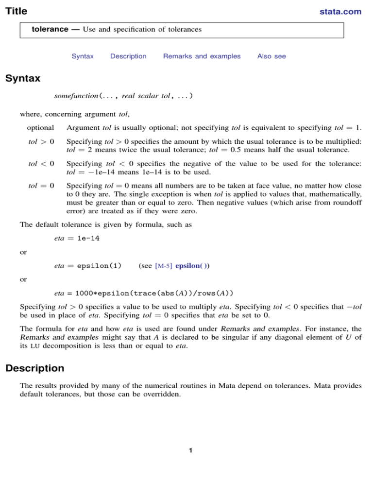
Title
stata.com
tolerance — Use and specification of tolerances
Syntax
Description
Remarks and examples
Also see
Syntax
somefunction(. . . , real scalar tol, . . . )
where, concerning argument tol,
optional
Argument tol is usually optional; not specifying tol is equivalent to specifying tol = 1.
tol > 0
Specifying tol > 0 specifies the amount by which the usual tolerance is to be multiplied:
tol = 2 means twice the usual tolerance; tol = 0.5 means half the usual tolerance.
tol < 0
Specifying tol < 0 specifies the negative of the value to be used for the tolerance:
tol = −1e–14 means 1e–14 is to be used.
tol = 0
Specifying tol = 0 means all numbers are to be taken at face value, no matter how close
to 0 they are. The single exception is when tol is applied to values that, mathematically,
must be greater than or equal to zero. Then negative values (which arise from roundoff
error) are treated as if they were zero.
The default tolerance is given by formula, such as
eta = 1e-14
or
eta = epsilon(1)
(see [M-5] epsilon( ))
or
eta = 1000*epsilon(trace(abs(A))/rows(A))
Specifying tol > 0 specifies a value to be used to multiply eta. Specifying tol < 0 specifies that −tol
be used in place of eta. Specifying tol = 0 specifies that eta be set to 0.
The formula for eta and how eta is used are found under Remarks and examples. For instance, the
Remarks and examples might say that A is declared to be singular if any diagonal element of U of
its LU decomposition is less than or equal to eta.
Description
The results provided by many of the numerical routines in Mata depend on tolerances. Mata provides
default tolerances, but those can be overridden.
1
2
tolerance — Use and specification of tolerances
Remarks and examples
stata.com
Remarks are presented under the following headings:
The problem
Absolute versus relative tolerances
Specifying tolerances
The problem
In many formulas, zero is a special number in that, when the number arises, sometimes the result
cannot be calculated or, other times, something special needs to be done.
The problem is that zero—0.00000000000—seldom arises in numerical calculation. Because of
roundoff error, what would be zero were the calculation performed in infinite precision in fact is
1.03948e–15, or −4.4376e–16, etc.
If one behaves as if these small numbers are exactly what they seem to be (1.03948e–15 is taken to
mean 1.03948e–15 and not zero), some formulas produce wildly inaccurate results; see [M-5] lusolve( )
for an example.
Thus routines use tolerances—preset numbers—to determine when a number is small enough to be
considered to be zero.
The problem with tolerances is determining what they ought to be.
Absolute versus relative tolerances
Tolerances come in two varieties: absolute and relative.
An absolute tolerance is a fixed number that is used to make direct comparisons. If the tolerance for
a particular routine were 1e–14, then 8.99e–15 in some calculation would be considered to be close
enough to zero to act as if it were, in fact, zero, and 1.000001e–14 would be considered a valid,
nonzero number.
But is 1e–14 small? The number may look small to you, but whether 1e–14 is small depends on
what is being measured and the units in which it is measured. If all the numbers in a certain problem
were around 1e–12, you might suspect that 1e–14 is a reasonable number.
That leads to relative measures of tolerance. Rather than treating, say, a predetermined quantity as
being so small as to be zero, one specifies a value (for example, 1e–14) multiplied by something and
uses that as the definition of small.
Consider the following matrix:
5.5e–15
1.3e–16
1.2e–16
6.4e–15
What is the rank of the matrix? One way to answer that question would be to take the LU decomposition
of the matrix and then count the number of diagonal elements of U that are greater than zero. Here,
however, we will just look at the matrix.
The absolutist view is that the matrix is full of roundoff error and that the matrix is really indistinguishable from the matrix
0 0
0 0
tolerance — Use and specification of tolerances
3
The matrix has rank 0. The relativist view is that the matrix has rank 2 because, other than a scale
factor of 1e–16, the matrix is indistinguishable from
55.0 1.2
1.3 64.0
There is no way this question can be answered until someone tells you how the matrix arose and the
units in which it is measured.
Nevertheless, most Mata routines would (by default) adopt the relativist view: the matrix is of full
rank. That is because most Mata routines are implemented using relative measures of tolerance, chosen
because Mata routines are mostly used by people performing statistics, who tend to make calculations
such as X 0 X and X 0 Z on data matrices, and those resulting matrices can contain very large numbers.
Such a matrix might contain
5.5e+14 1.2e+12
1.3e+13 2.4e+13
Given a matrix with such large elements, one is tempted to change one’s view as to what is small.
Calculate the rank of the following matrix:


5.5e+14 1.2e+12 1.5e–04
 1.3e+13 2.4e+13 2.8e–05 
1.3e–04 2.4e–05 8.7e–05
This time, we will do the problem correctly: we will take the LU decomposition and count the number
of nonzero entries along the diagonal of U. For the above matrix, the diagonal of U turns out to be
(5.5e+14, 2.4e+13, 0.000087).
An absolutist would tell you that the matrix is of full rank; the smallest number along the diagonal of
U is 0.000087 (8.7e–5), and that is still a respectable number, at least when compared with computer
precision, which is about 2.22e–16 (see [M-5] epsilon( )).
Most Mata routines would tell you that the matrix has rank 2. Numbers such as 0.000087 may seem
respectable when compared with machine precision, but 0.000087 is, relatively speaking, a very small
number, being about 4.6e–19 relative to the average value of the diagonal elements.
Specifying tolerances
Most Mata routines use relative tolerances, but there is no rule. You must read the documentation for
the function you are using.
When the tolerance entry for a function directs you here, [M-1] tolerance, then the tolerance works as
summarized under Syntax above. Specify a positive number, and that number multiplies the default;
specify a negative number, and the corresponding positive number is used in place of the default.
Also see
[M-5] epsilon( ) — Unit roundoff error (machine precision)
[M-5] solve tol( ) — Tolerance used by solvers and inverters
[M-1] intro — Introduction and advice