Hierarchical Multiple Regression in SPSS
This example shows you how to perform hierarchical multiple regression, a variant of the
basic multiple regression procedure that allows you to specify a fixed order of entry for variables
in order to control for the effects of covariates or to test the effects of certain predictors
independent of the influence of others.
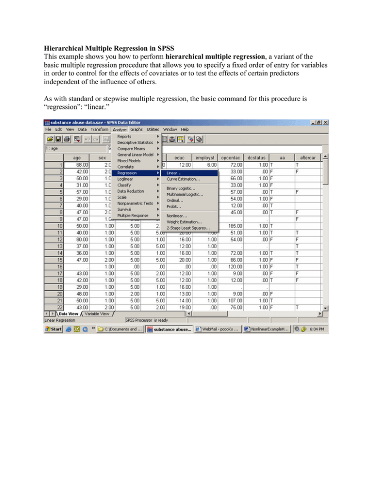
As with standard or stepwise multiple regression, the basic command for this procedure is
“regression”: “linear.”
In the main dialog box, input the dependent variable. In this case, looking at data from a
substance abuse treatment program (the same data as in the stepwise multiple regression
example), we want to predict amount of treatment that a patient receives (hours of outpatient
contact, or “opcontact”).
Next, enter a set of predictor variables into this box. These are the variables that you want SPSS
to put into the model first – generally the ones that you want to control for when testing the
variables that you are truly interested in. For instance, in this analysis, I want to find out whether
employment status predicts the number of sessions of treatment that someone receives, but I am
concerned that other variables like socioeconomic status, age, or race/ethnicity might be
associated with both employment status and hours of outpatient contact. To make sure that these
variables do not explain away the entire association between employment status and hours of
treatment, I put them into the model first. This ensures that they will get “credit” for any shared
variability that they may have with the predictor that I am really interested in, employment
status. Any observed effect of employment status can then be said to be “independent of” the
effects of these variables that I have already controlled for.
The next step is to input the variable that I am really interested in, which is employment status.
To put it into the model, click the “next” button. You will see all of the predictor variables that
you previously entered disappear – don’t panic! They are still in the model, just not on the
current screen.
The “Next” button clears out the
list of independent variables
from your first step, and lets you
enter the next “block” of
predictors. This order-of-entry
feature, where some predictors
are considered before looking at
others, is what makes this a
“hierarchical” regression
procedure – some variables take
precedence in the hierarchy over
others, based on the order in
which you enter them into the
model.
Now hit the “OK” button to run the analysis. You could also hit “Next” again, if you wanted to
enter a third (or fourth, or fifth, etc.) block of variables. Often researchers will enter variables as
related sets – for example, all demographic variables in a first step, all potentially confounding
psychological variables in a second step, and then the variable that you are most interested in as a
third step. This is not necessarily the only way to proceed – you could also enter each variable as
a separate step if that seems more logical based on the design of your experiment. SPSS also lets
you specify a “Method” for each step – for example, if you wanted to know which demographic
predictors were most effective, you could use a stepwise procedure in the first block, and then
still enter employment status in the second block. To do this, you would just choose “Forward
Stepwise” instead of “Enter” from the drop-down box labeled “Method.”
Using just the default “Enter” method, with all the variables in Block 1 (demographics) entered
together, followed by employment status as a predictor in Block 2, we get the following output:
Variables Entered/Removedb
Model
1
2
Variables
Entered
educ, sex,
ethnic,
marstat,
a
age
employst a
Variables
Removed
Method
.
Enter
.
Enter
a. All requested variables entered.
b. Dependent Variable: opcontac
This table confirms which variables were entered in each step – the five demographic variables
in step 1, and employment status in step 2.
Model Summary
Model
1
2
R
.348a
.353b
R Square
.121
.125
Adjusted
R Square
.043
.029
Std. Error of
the Estimate
34.94411
35.18930
a. Predictors: (Constant), educ, sex, ethnic, marstat, age
b. Predictors: (Constant), educ, sex, ethnic, marstat, age,
employst
The next table shows you the percent of variability in the dependent variable that can be
accounted for by all the predictors together (that’s the interpretation of R-square). The change in
R2 is a way to evaluate how much predictive power was added to the model by the addition of
another variable in step 2. In this case, the % of variability accounted for went up from 12.1% to
12.5% – not much of an increase.
ANOVAc
Model
1
2
Regression
Residual
Total
Regression
Residual
Total
Sum of
Squares
9420.339
68381.080
77801.419
9695.649
68105.770
77801.419
df
5
56
61
6
55
61
Mean Square
1884.068
1221.091
F
1.543
Sig.
.191a
1615.942
1238.287
1.305
.270b
a. Predictors: (Constant), educ, sex, ethnic, marstat, age
b. Predictors: (Constant), educ, sex, ethnic, marstat, age, employst
c. Dependent Variable: opcontac
This table confirms our suspicions: Neither the first model (demographic variables alone) nor the
second model (demographics plus employment status) predicted scores on the DV to a
statistically significant degree. (Look in the “sig” column for p-values, which need to be below
.05 to say that you have a statistically significant result). If the first set of predictors was
significant, but the second wasn’t, it would mean that employment did not have an effect above
and beyond the effects of demographics. Unfortunately, in this case, none of the predictors are
significant.
Coefficientsa
Model
1
2
(Constant)
age
sex
ethnic
marstat
educ
(Constant)
age
sex
ethnic
marstat
educ
employst
Unstandardized
Coefficients
B
Std. Error
-12.736
28.290
.153
.386
-4.607
11.870
5.531
3.462
.384
2.693
2.521
1.503
-12.601
28.490
.141
.390
-5.968
12.297
5.319
3.515
.198
2.740
2.595
1.522
1.613
3.421
Standardized
Coefficients
Beta
.054
-.050
.209
.019
.225
.050
-.064
.201
.010
.231
.063
t
-.450
.397
-.388
1.598
.143
1.677
-.442
.362
-.485
1.513
.072
1.705
.472
Sig.
.654
.693
.699
.116
.887
.099
.660
.719
.629
.136
.943
.094
.639
a. Dependent Variable: opcontac
This “coefficients” table would be useful if some of our predictors were statistically significant.
In this case, since they weren’t, the coefficients aren’t interpretable. If the predictors had been
statistically significant, these betas (B) are the weights that you could multiply each individual
person’s scores on the independent variables by, in order to obtain that individual’s predicted
score on the dependent variable.