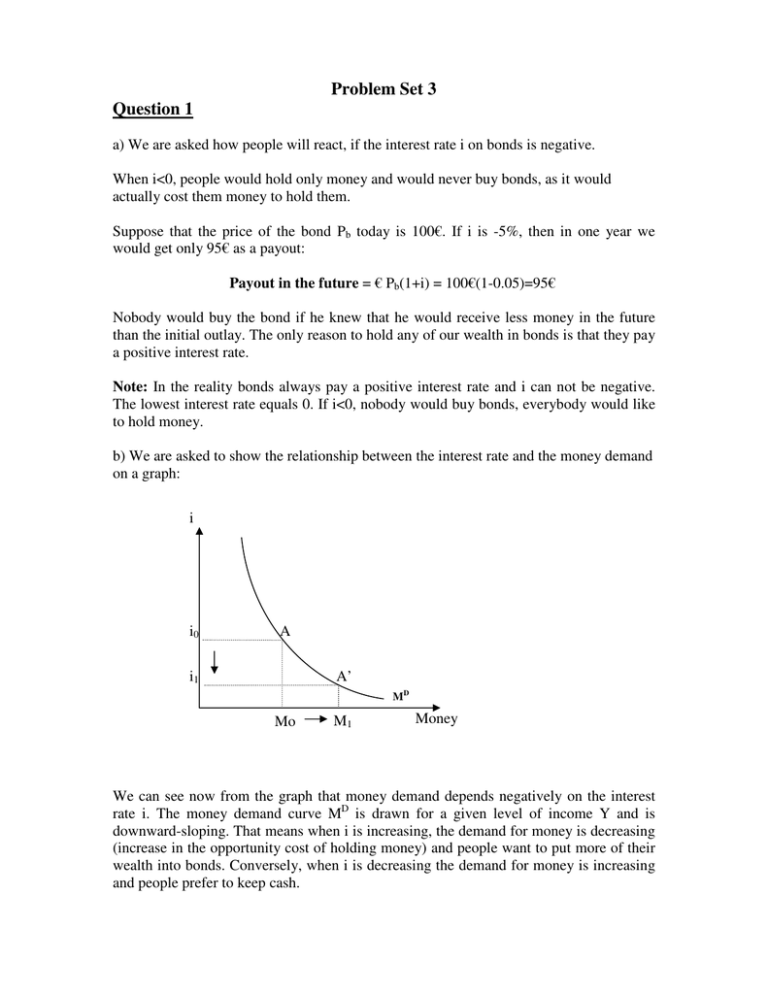
Problem Set 3
Question 1
a) We are asked how people will react, if the interest rate i on bonds is negative.
When i<0, people would hold only money and would never buy bonds, as it would
actually cost them money to hold them.
Suppose that the price of the bond Pb today is 100€. If i is -5%, then in one year we
would get only 95€ as a payout:
Payout in the future = € Pb(1+i) = 100€(1-0.05)=95€
Nobody would buy the bond if he knew that he would receive less money in the future
than the initial outlay. The only reason to hold any of our wealth in bonds is that they pay
a positive interest rate.
Note: In the reality bonds always pay a positive interest rate and i can not be negative.
The lowest interest rate equals 0. If i<0, nobody would buy bonds, everybody would like
to hold money.
b) We are asked to show the relationship between the interest rate and the money demand
on a graph:
i
i0
A
i1
A’
MD
Mo
M1
Money
We can see now from the graph that money demand depends negatively on the interest
rate i. The money demand curve MD is drawn for a given level of income Y and is
downward-sloping. That means when i is increasing, the demand for money is decreasing
(increase in the opportunity cost of holding money) and people want to put more of their
wealth into bonds. Conversely, when i is decreasing the demand for money is increasing
and people prefer to keep cash.
c) First we are asked to derive the LM curve:
Suppose, that for some reason output Y is decreasing from Y0 to Y1 (Graph 2), so that
money demand curve shifts to the left from MD to MD’ (Graph1). But because money
supply MS is fixed, the interest rate decreases from i0 to i1 in order to keep the money
market in equilibrium. So we can see now, that a decrease in output leads to a decrease in
the interest rate and to a new equilibrium at point A’. We have positive relationship
between Y and i, represented by our upward-sloping LM curve (Graph2).
(1) Money Market Only
i
(2) Both Money Market and Goods Market
MS
i
i0
A
i0
i1
A’
i1
MD’
M0
P
LM
A
A’
MD
M
P
Y1
Y0
Y
But how will LM curve look if the interest rate is very close to zero? (See diagram
below)
Here we have first the same case: Because of decreasing of Y from Y0 to Y1 our money
demand MD is decreasing causing a fall in the interest rate form i0 to i1 and new equilibrium
at point A’.
Suppose now that output decreases even more from Y1 to Y2. Money demand decreases and
the MD curve shifts further to the left. But now the equilibrium on the Money Market is at
point A’’ with i = 0. When i reaches zero people are now indifferent if they hold money or
bonds. Both money and bonds pay the same interest rate, so they are willing to hold more
money and therefore fewer bonds. Even, if Y is decreasing below Y2, people still demand
more money at the same interest rate so that our LM curve is flat for points left of the
equilibrium point A’’. Here i has no impact on Y. Because of i=0, there is a ‘liquidity trap’.
i
MS
i
i0
A
i0
i1
A’
i1
i2
A’’
i2
MD’’’ MD’
MD
LM
A
A’
A’’
Y2
M
P
M
P
Y1
Y0
Y
(d) Expansionary monetary policy: MS and the interest rate is very close to zero
Suppose, we are at point A with output Y0 and interest rate i0 (which is already very low) and
central bank increases now MS to MS’.
In the first step, if money supply is increasing, the interest rate is decreasing to i1 in order to
bring money market back to equilibrium (Graph 1). Because of decrease in i, investment in
the goods market is increasing and output increases to Y1 and the new equilibrium is A’
(Graph 2).
In the second step, the central bank increases MS’ further to MS’’. But at point A’ the
interest rate i1 is already zero and people want to hold more money at the same i. At i=0 the
LM’’curve is flat. The interest rate does not change and investment does not change either
and output does not increase. Monetary policy has fallen into the “Liquidity Trap”. The
increase in money supply can not increase output and economy remains at point A’ (Graph
2).
(2) Both Money Market and Goods Market
(1) Money Market Only
i
i0
i1
MD
MS
M S’
i
MS’’
A
i0
A’
M 0 M1
P P
A’’
M2
P
M
P
i1
IS
LM
LM’
LM’’
A
A’
Y0
Y1
Y
(e) The question: How effective is expansionary monetary policy at the interest rate i=0, we
have already answered in point (d): the policy is not effective because it falls into the
“Liquidity Trap”: an increase in Ms has no effect on i or on Y.
Expansionary fiscal policy: G or T
when the interest rate is very close to zero
If government spending is increasing or taxes are decreasing, the IS curve (representing
goods market) shifts to the right and causes an increase in output from Y0 to Y1 (Note: we
have here no crowding-out effect because LM is flat). If we have a further increase in G or
decrease in T, the IS curve shifts further to the right. Output increases further from Y1 to Y2
and finally we can get the economy out of liquidity trap.
i
IS
IS’
IS’’
A’’
i1
i0
LM
A
Y0
A’
Y1
Y2
Y
Comparison: Expansionary monetary policy and LM curve is flat
If LM curve is flat, the expansionary monetary policy is not effective. If MS is increasing, the
interest rate is not increasing because interest elasticity of MD is infinite, in other words MD
is very sensitive to interest rate which does not change. No increase in i causes no increase in
investment, and therefore no increase in output.
In the presence of liquidity trap LM curve is also flat for the same i=0 and the policy causes
no increase in output, so that the policy is not effective.
Comparison: Expansionary fiscal policy and LM curve is flat
If the LM curve is flat, the expansionary fiscal policy is always effective. If government
spending is increasing or taxes are decreasing, the IS curve shifts to the right and causes an
increase in output. Because the money demand is infinitely elastic, the interest rate does not
change and there is no decrease in investment and no crowding-out effect at all.
In the presence of the liquidity trap LM curve is also flat for the same i=0 and the policy
causes an increase in output, so that it is effective.
Conclusion:
If the interest rate does not change, the intervention in the goods market through the
expansionary fiscal policy, is effective, but the intervention in the money market, through
the expansionary monetary policy, is not effective!
Problem Set 3
Question 2
The equilibrium condition for the Labour Market is given by following equation:
F (u n , z ) =
1
1+ µ
a) We are asked to draw the price setting equation and wage setting equation on the
graph:
Real wage W/P
Equilibrium
wage rate
W
1
=
P 1+ µ
A
Price-Setting relation (PS)
Wage-Setting relation (WS)
un
Unemployment rate u
Natural rate of
unemployment
Derivation of Wage-Setting Equation (Worker/Labour Side):
Assumption: P is a given actual price level
Nominal wage:
W = P ⋅ F (u , z )
If we divide both sides of the equation by P, we get:
W
= F (u , z ) , which is the WS equation
P
( −,+)
W
is real wage (nominal wage divided by a given price level P), which tells us
P
how many goods an employee can buy with her nominal wage; u is the unemployment
rate and z is an exogenous variable that denotes other factors (e.g. unemployment
Here,
benefits, employment protection, minimum wages) which determine the real wage given
P and u.
Summary: The WS equation characterizes wage determination in the Labour Market. It
is drawn on the graph as the downward-sloping curve and it shows a negative relationship
between the unemployment rate and the real wage. This means; the higher the
unemployment rate, the less bargaining power employees have and so the lower the real
wage that will be chosen by wage setters. There is a positive relation between parameter z
and the real wage. If z is increasing, the bargaining power of employees is increasing and
the real wage is increasing as well.
Derivation of Price-Setting Equation (Firm Side):
Assumptions:
• The goods market is not perfectly competitive and firms set prices higher than
Marginal Costs (MC)
• Labour is the only factor of production and MC=W
P = (1 + µ ) MC
P = (1 + µ )W
Here, µ is the markup on the price over costs. Price exceeds the marginal cost W by a
factor equal 1+µ. (Note: If goods market is perfectly competitive: µ= 0 and p=MC=W.)
If we divide now both sides of the equation by P and then by (1+µ), we get:
W
1
, which is the PS equation
=
P 1+
Summary: The PS equation characterizes price determination in the Labour Market. It
shows the negative relationship between the real wage and the markup set by the firms.
The higher the markup, the lower the real wage will be. The PS relation is drawn on the
graph as the horizontal line. The real wage implied by the price setting relation does not
depend on the unemployment rate. For example if the unemployment rate increases, the
real wage implied by price setting relation does not change.
(b) We are asked to show equilibrium parameters.
The equilibrium is given at point A. Here the WS relation equals the PS relation:
1
F (u n , z ) =
1+ µ
1
The equilibrium real wage is
and the equilibrium unemployment rate is un,
1+ µ
which is called the natural rate of unemployment. In other words, un is the
unemployment rate such that the real wage
real wage
W
implied by the price setting.
P
W
chosen in the wage setting is equal to the
P
(c) We are asked, what will happen to un, if the government increases the employment
protection, denoted as z in the WS equation.
An example of employment protection: Employers have to give a long period of notice
when dismissing a worker.
W/P
1
1+ µ
A
A’
PS
WS’
WS
un
u
un ’
If at a given P and a given un, employment protection (represented by z) increases, the
employees have more bargaining power because they are less afraid of the possibility of
being made unemployed. As the bargaining power of employees increases, they will
demand an increase in their real wages. The WS curve shifts up. But the firms are willing
to pay only the real wage which is not bigger than
1
. The unemployment rate has to
1+ µ
increase from un to un’ to keep the real wage at the level given by
1
. The economy
1+ µ
moves right along the PS line from A to A’, a new equilibrium in the Labour Market,
where the equilibrium real wage has not changed,
unemployment rate is un’ where un’> un.
1
, and the new equilibrium
1+ µ
Summary: An increase in employment protection causes an increase in the natural rate
of unemployment, but has no effect on the real wage.
(d) Now we are asked, what will happen to un, if parliament adopts a stronger antitrust
law, which aims to increase the market competition. This is captured in the parameter µ
in the PS equation.
An example of antitrust law: European Union liberalization of the goods market that
reduces the monopoly power of the existing firms selling in the EU.
W/P
1
1+ µ'
A’
PS’
A
1
1+ µ
PS
WS
un ’
un
u
Because of increased competition in the market, the market power of firms is decreasing
and so leads to a decrease in their markup µ. A decrease in markup shifts the PS line up
given un and given P, so that the real wage set by firms increases from
1
1
to
.
1+ µ
1+ µ'
This increase in the real wage causes the natural rate of unemployment to decreasing
from un to un’. The economy moves left along the WS curve from A to A’, a new
equilibrium in the Labour Market, where the new equilibrium real wage is
1
1
>
and the new equilibrium unemployment rate is un’< un.
1+ µ' 1+ µ
Summary: An increase in market competition caused by stronger antitrust legislation
increases the real wage and decreases the natural rate of unemployment.