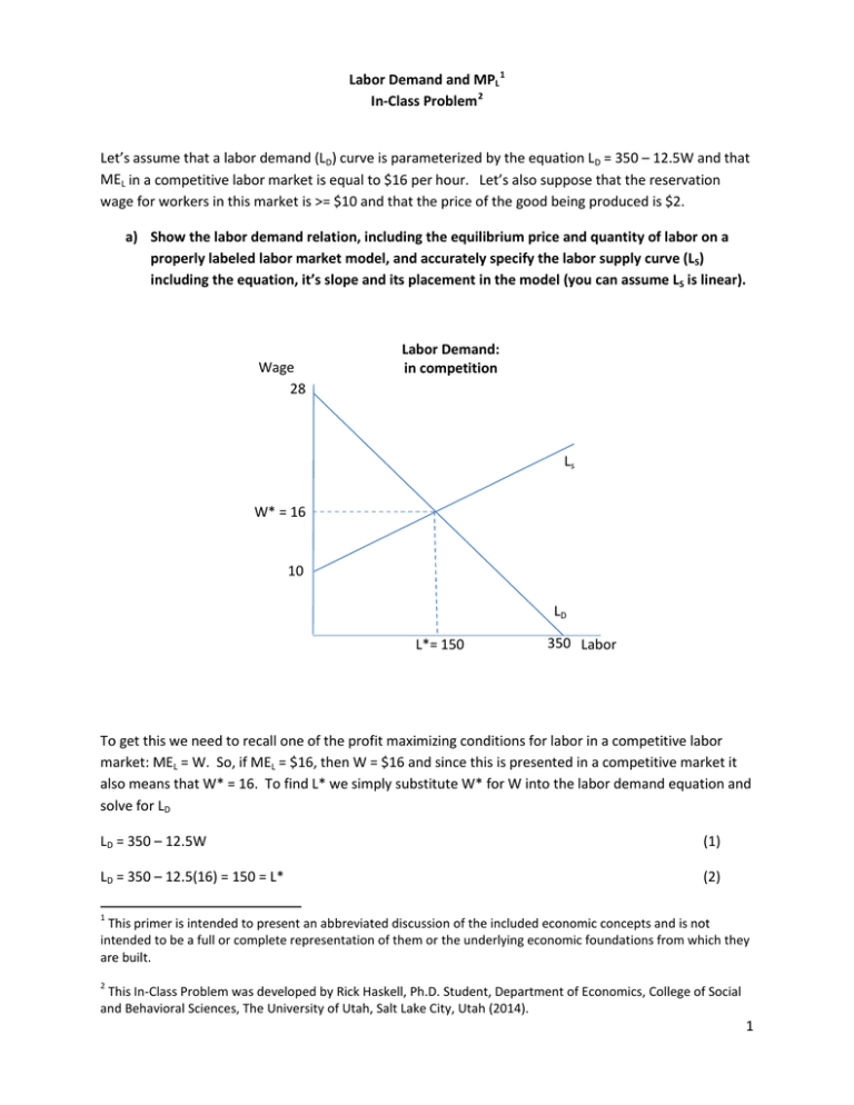
Labor Demand and MPL 1
In-Class Problem 2
Let’s assume that a labor demand (LD) curve is parameterized by the equation LD = 350 – 12.5W and that
MEL in a competitive labor market is equal to $16 per hour. Let’s also suppose that the reservation
wage for workers in this market is >= $10 and that the price of the good being produced is $2.
a) Show the labor demand relation, including the equilibrium price and quantity of labor on a
properly labeled labor market model, and accurately specify the labor supply curve (LS)
including the equation, it’s slope and its placement in the model (you can assume LS is linear).
Wage
28
Labor Demand:
in competition
Ls
W* = 16
10
LD
L*= 150
350 Labor
To get this we need to recall one of the profit maximizing conditions for labor in a competitive labor
market: MEL = W. So, if MEL = $16, then W = $16 and since this is presented in a competitive market it
also means that W* = 16. To find L* we simply substitute W* for W into the labor demand equation and
solve for LD
LD = 350 – 12.5W
(1)
LD = 350 – 12.5(16) = 150 = L*
(2)
1
This primer is intended to present an abbreviated discussion of the included economic concepts and is not
intended to be a full or complete representation of them or the underlying economic foundations from which they
are built.
2
This In-Class Problem was developed by Rick Haskell, Ph.D. Student, Department of Economics, College of Social
and Behavioral Sciences, The University of Utah, Salt Lake City, Utah (2014).
1
Since we’re told that the reservation wage is >= $10, this tells us that at or below $10, workers aren’t
willing to work. Since these workers are the supply of labor this gives us a hint as to where the labor
supply curve intersects the Wage axis, at 10.
We know that the slope of LS =
rise
and
run
we can see from the graph we completed with the given data,
that LS rises from 10 to 16 as labor changes from 0 to 150, which equates to a
𝑊2 −𝑊1
𝐿2 −𝐿1
=
16−10
150−0
=
6
150
So the slope of labor supply is
1
.
25
If we’ve determined the intercept on the Wage axis is 10 and the slope is
yields an in labor supply equation of
W = 10 +
1
,
25
rise
as
run
follows:
(3)
then we know that this
1
L
25 S
(4)
Which can be rearranged as:
LS = 25W – 250
(5)
We can check this by seeing if it yields the same equilibrium levels of wage and labor that we got earlier
LS = L D
(6)
25W – 250 = 350 – 12.5W
37.5W = 600
W= 16 ; which is exactly what we expected!
b) Now, what is the marginal product of labor (MPL) at equilibrium in this market?
If MEL = $16 in a competitive market then it also means that MEL = MRPL, which is the profit maximizing
condition for labor in a competitive market. So we can work backwards from this to find MPL given that
we know MRPL = MPL x P, and price was given as $2.
MEL = MRPL = (MPL)(P)
(7)
16 = (MPL)(2)
MPL = 8
2
c) What might this look like on a Total Product of Labor graph?
We don’t know much about this particular Total Product of Labor model with the information given, but
what we do know is that we want to hire the number of workers at which MRPL = MEL (general
condition) or MRPL = W (competitive market condition since MEL = W in a competitive market). In this
case, if MPL = 8 at W = 8 and L = 150, we can suppose that MPL < 0 when we hire the next worker,
which simply means that MPL has change from positive to negative as we go from 150 workers to 151
workers.
Generally, the Marginal Labor Productivity model will look like this:
Marginal Labor Productivity
(holding capital fixed)
Marginal
Product
of Labor
MPL = 8
0
Increasing
Returns to Scale
L= 150
L= 151 Decreasing
Labor
Returns to Scale
Total Labor Productivity
(holding capital fixed)
Total
Product
of Labor
Slope = 0
MPL = 8
Increasing
Returns to Scale
L= 150
L= 151
Decreasing
Labor
Returns to Scale
3