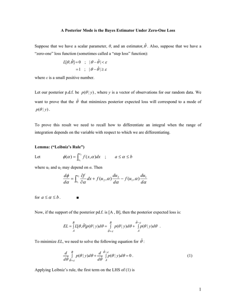
A Posterior Mode is the Bayes Estimator Under Zero-One Loss
Suppose that we have a scalar parameter, θ, and an estimator, ˆ . Also, suppose that we have a
“zero-one” loss function (sometimes called a “step loss” function):
L[ ,ˆ]  0 ; |   ˆ |  
 1 ; |   ˆ |  
where ε is a small positive number.
Let our posterior p.d.f. be p ( | y ) , where y is a vector of observations for our random data. We
want to prove that the ˆ that minimizes posterior expected loss will correspond to a mode of
p ( | y ) .
To prove this result we need to recall how to differentiate an integral when the range of
integration depends on the variable with respect to which we are differentiating.
Lemma: (“Leibniz’s Rule”)
Let
u2
 ( )   f ( x,  )dx ;
a  b
u1
where u1 and u2 may depend on α. Then
u 2 f
du
du
d

dx  f (u 2 ,  ) 2  f (u1 ,  ) 1
u1 
d
d
d
for a    b .
■
Now, if the support of the posterior pd.f. is [A , B], then the posterior expected loss is:
B
B
ˆ 
A
ˆ  
A
EL   L[ ,ˆ]p ( | y )d   p ( | y )d   p( | y ) d .
To minimize EL, we need to solve the following equation for ˆ :
ˆ
d B
d  
p ( | y )d 

 p ( | y )d  0 .
dˆ ˆ  
dˆ A
(1)
Applying Leibniz’s rule, the first term on the LHS of (1) is
1
B

ˆ  
which is just
d
dB
d (ˆ   )
 p (ˆ   | y )
p ( | y )d  p ( B | y )
,
dˆ
dˆ
dˆ
 p (ˆ   | y ) .
Applying Leibniz’s rule, the second term on the LHS of (1) is
ˆ 

A
which is just
d
d (ˆ   )
dA
 p( A | y)
p( | y ) d  p(ˆ   | y )
,
ˆ
ˆ
d
d
dˆ
p(ˆ   | y ) .
So, the condition in (1) becomes:
p (ˆ   | y )  p (ˆ   | y ) .
(2)
The value of ˆ that satisfies (2) can be found graphically, as follows (Leonard and Hsu, 1999,
pp.158-159):
1. Plot the posterior pd.f., and suppose that it is uni-modal.
2. Choose a small positive value for ε.
3. Draw a horizontal line, parallel to the θ axis. Raise or lower the line until the distance
between the two points where the line intersects p ( | y ) is 2ε.
4. Drop a vertical line down from the mid-point of this line of length 2ε, so that it crosses
the horizontal axis at   ˆ .
5. If ε is made arbitrarily small, then ˆ will locate the mode of the posterior pd.f.
Note that if the posterior is both uni-modal and symmetric, then this method will locate the mode
for any (positive) choice of ε. In this case, of course the mode, median and mean (if it exists) of
the posterior p.d.f. will all coincide.
If the posterior density is multi-modal, the method above will locate local turning points in the
density. Which turning points are found will depend on the choice of ε. In the multi-modal case,
the value of the posterior expected loss will have to be computed for each “solution”, and this will
determine the choice of ˆ .
Figure 1 illustrates this procedure for the (asymmetric) uni-model case; and Figure 2 illustrates it
for the case of a bi-modal posterior density. The latter is a mixture of two normals, with means of
1 and 4, and unit variances. The weights are 0.38 and 0.62 respectively. In Figure 2, the two
modes occur at ˆ  1 and ˆ  4 . There is a local minimum at ˆ  2.2 . It can be shown
1
3
2
(Leonard and Hsu, 1999, p.158) that in this particular case the value of the posterior
expected loss is least when ˆ3  4 is chosen as the estimator of θ.
Reference
Leonard, T. and J. S. J. Hsu (1999). Bayesian Methods. Cambridge University Press, Cambridge.
2
Figure 1: Uni-Modal Posterior p.d.f.
0.30
0.25
p(θ|y)
0.20
width = 2ε
0.15
0.10
Bayes estimator
0.05
0.00
0
1
2
3
4
5
6
7
8
9
10
θ
0.3
Figure 2: Multi‐Modal Posterior p.d.f.
0.25
width = 2ε
p(θ|y)
0.2
0.15
0.1
0.05
θ
0
‐4
‐2
0
2
4
6
8
10
David E. Giles. Department of Economics, University of Victoria
3