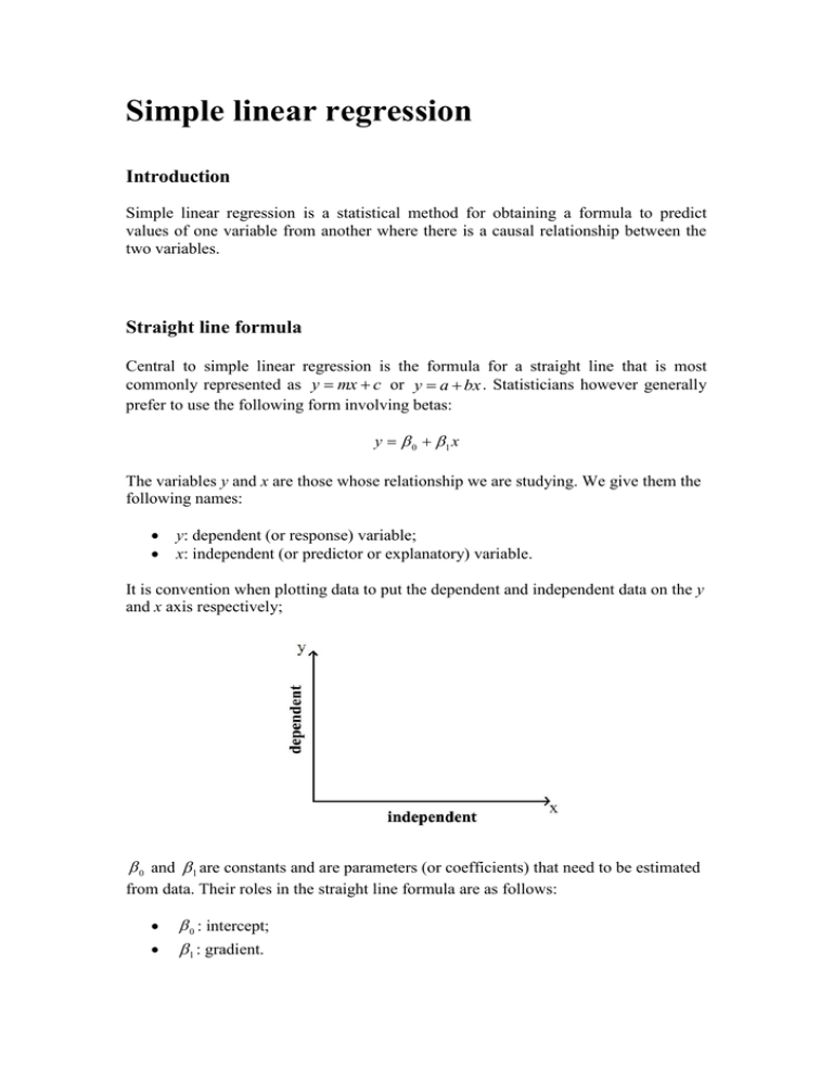
Simple linear regression
Introduction
Simple linear regression is a statistical method for obtaining a formula to predict
values of one variable from another where there is a causal relationship between the
two variables.
Straight line formula
Central to simple linear regression is the formula for a straight line that is most
commonly represented as y  mx  c or y  a  bx . Statisticians however generally
prefer to use the following form involving betas:
y   0  1 x
The variables y and x are those whose relationship we are studying. We give them the
following names:


y: dependent (or response) variable;
x: independent (or predictor or explanatory) variable.
It is convention when plotting data to put the dependent and independent data on the y
and x axis respectively;
 0 and  1 are constants and are parameters (or coefficients) that need to be estimated
from data. Their roles in the straight line formula are as follows:


 0 : intercept;
 1 : gradient.
For instance the line y  1 0.5x has an intercept of 1 and a gradient of 0.5. Its graph
is as follows:
Model assumptions
In simple linear regression we aim to predict the response for the ith individual, Yi ,
using the individual‟s score of a single predictor variable, X i . The form of the model is
given by:
Yi   0  1 X i   i
which comprises a deterministic component involving the two regression coefficients
(  0 and  1 ) and a random component involving the residual (error) term (  i ).
The deterministic component is in the form of a straight line which provides the
predicted (mean/expected) response for a given predictor variable value.
The residual terms represent the difference between the predicted value and the
observed value of an individual. They are assumed to be independently and
identically distributed normally with zero mean and variance  2 , and account for
natural variability as well as maybe measurement error. Our data should thus appear
to be a collection of points that are randomly scattered around a straight line with
constant variability along the line:
The deterministic component is a linear function of the unknown regression
coefficients which need to be estimated so that the model „best‟ describes the data.
This is achieved mathematically by minimising the sum of the squared residual terms
(least squares). The fitting also produces an estimate of the error variance which is
necessary for things like significance test regarding the regression coefficients and for
producing confidence/prediction intervals.
Example
Suppose we are interested in predicting the total dissolved solids (TDS)
concentrations (mg/L) in a particular river as a function of the discharge flow (m3/s).
We have collected data that comprise a sample of 35 observations that were collected
over the previous year.
The first step is to look carefully at the data:



Is there an upwards/downwards trend in the data or could a horizontal line be
fit though the data?
Is the trend linear or curvilinear?
Is there constant variance along the regression line or does it systematically
change as the predictor variable changes?
700
Total dissolved solids conc
600
500
400
300
200
0
2000
4000
6000
8000
Discharge flow
The scatterplot above suggests that there is a downwards trend in the data, however
there is a curvilinear relationship. The variance about a hypothetical curve appears
fairly constant.
Transformations
Simple linear regression is appropriate for modelling linear trends where the data is
uniformly spread around the line. If this is not the case then we should be using other
modelling techniques and/or transforming our data to meet the requirements. When
considering transformations the following is a guide:


If the trend is curvilinear consider a transformation of the predictor variable, x.
If constant variance is a problem (and maybe curvilinear as well) consider
either a transformation of the response variable, y, or a transformation of both
the response and the predictor variable, x and y.
Tukey‟s “bulging rule” can act as a guide to selecting power transformations.
Compare your data to the above and if it has the shape in any of the quadrants then
consider the transformations where:


up – use powers of the variable greater than 1 (e.g. x2, etc);
down - powers of the variable less than 1 (e.g. log(x), 1/x, √x etc).
Note, sometimes a second application of Tukey‟s bulging rule is necessary to gain
linearity with constant variability.
Example (revisited)
Returning to our example, the scatterplot reveals the data to belong to the bottom left
quadrant of Tukey‟s bulging rule. Since the variance about a hypothetical curve
appears fairly constant, thus we shall try transforming just the predictor variable.
Tukey‟s bulging rule suggests a “down” power; we shall try the log natural
transformation first
The resulting scatterplot of TDS against ln(Discharge) is now far more satisfactory:
700
Total dissolved solids conc
600
500
400
300
200
5.00
6.00
7.00
8.00
ln(Discharge flow)
The data now appears to be suitable for simple linear regression and we shall now
consider selected output from the statistics package SPSS.
Correlations
Total
dissolved
solids conc
Pearson Correlation
Sig. (1-tailed)
N
Total dissolved
solids conc
ln(Discharge flow)
Total dissolved
solids conc
ln(Discharge flow)
Total dissolved
solids conc
ln(Discharge flow)
ln(Discharge
flow)
1.000
-.735
-.735
1.000
.
.000
.000
.
35
35
35
35
The correlations table displays Pearson correlation coefficients, significance values,
and the number of cases with non-missing values. As expected we see that we have a
strong negative correlation (-.735) between the two variables. From the significance
test p-value we can see that we have very strong evidence (p<0.001) to suggest that
there is a linear correlation between the two variables.
9.00
Model Summaryb
Model
1
R
.735a
R Square
.540
Adjusted
R Square
.526
Std. Error of
the Estimate
78.261
a. Predictors: (Constant), ln(Discharge flow)
b. Dependent Variable: Total dissolved solids conc
The model summary table displays:




R, the multiple correlation coefficient, is a measure of the strength of the
linear relationship between the response variable and the set of explanatory
variables. It is the highest possible simple correlation between the response
variable and any linear combination of the explanatory variables. For simple
linear regression where we have just two variables, this is the same as the
absolute value of the Pearson‟s correlation coefficient we have already seen
above. However, in multiple regression this allows us to measure the
correlation involving the response variable and more than one explanatory
variable.
R squared is the proportion of variation in the response variable explained by
the regression model. The values of R squared range from 0 to 1; small values
indicate that the model does not fit the data well. From the above we can see
that the model fits the data reasonably well; 54% of the variation in the TDS
values can be explained by the fitted line together with the lnDischarge
values. R squared is also known as the coefficient of determination.
The R squared value can be over optimistic in its estimate of how well a
model fits the population; the adjusted R square value is attempts to correct for
this. Here we can see it has slightly reduced the estimated proportion. If you
have a small data set it may be worth reporting the adjusted R squared value.
The standard error of the estimate is the estimate of the standard deviation of
the error term of the model,  . This gives us an idea of the expected
variability of predictions and is used in calculation of confidence intervals and
significance tests.
Coefficientsa
Model
1
(Constant)
ln(Discharge flow)
Unstandardized
Coefficients
B
Std. Error
1103.967
105.320
-101.275
16.281
Standardized
Coefficients
Beta
-.735
t
10.482
-6.221
Sig.
.000
.000
95% Confidence Interval for B
Lower Bound
Upper Bound
889.693
1318.242
-134.399
-68.152
a. Dependent Variable: Total dissolved solids conc
The unstandardized coefficients are the coefficients of the estimated regression
model. Thus the expected TDS value is given by:
TDS  1103.967  101.275ln(Discharge) .
Thus we can see that for each one unit increase in ln(Discharge), the TDS value is
expected to decrease by 101.275 units. The intercept for this example could be
interpreted as the TDS value (1103.967) when the ln(Discharge) flow is zero (i.e.
Discharge = 1 m3/s.
The standardized coefficients are appropriate in multiple regression when we have
explanatory variables that are measured on different units. These coefficients are
obtained from regression after the explanatory variables are all standardized. The idea
is that the coefficients of explanatory variables can be more easily compared with
each other as they are then on the same scale. In simple linear regression they are of
little concern.
The standard errors give us estimates of the variability of the (unstandardised)
coefficients and are used for significance tests for the coefficients and for the
displayed 95% confidence intervals. The t values and corresponding significance
vales are tests assessing the worth of the (unstandardised) coefficients. It is usually of
importance to be assessing the worth of our predictor variable and hence evaluating
the significance of the coefficient  1 in our model formulation. That is we are
assessing for evidence of a significant non-zero slope. If the coefficient is not
significantly different to zero then this implies the predictor variable does not
influence our response variable.
Here we have both test are highly significant (p<0.001), indicating that we have very
strong evidence of need both the coefficients in our model. The resulting confidence
intervals expand our understanding of the problem. For example, with 95%
confidence we believe that the interval between -134.399 and -68.152 covers the true
unknown TDS value change per ln(Discharge) unit.
The remaining output is concerned with checking the model assumptions of
normality, linearity, homoscedasticity and independence of the residuals. Residuals
are the differences between the observed and predicted responses. The residual
scatterplots allow you to check:



Normality: the residuals should be normally distributed about the predicted
responses;
Linearity: the residuals should have a straight line relationship with the
predicted responses;
Homoscedasticity: the variance of the residuals about predicted responses
should be the same for all predicted responses.
Residuals Statisticsa
Predicted Value
Residual
Std. Predicted Value
Std. Residual
Minimum
198.53
-128.404
-3.060
-1.641
Maximum
558.19
214.702
1.248
2.743
Mean
454.00
.000
.000
.000
a. Dependent Variable: Total dissolved solids conc
Std. Deviation
83.491
77.101
1.000
.985
N
35
35
35
35
The above table summarises the predicted values and residuals in unstandarised and
standardised forms. It is usual practice to consider standardised residuals due to their
ease of interpretation. For instance outliers (observations that do not appear to fit the
model that well) can be identified as those observations with standardised residual
values above 3.3 (or less than -3.3). From the above we can see that we do not appear
to have any outliers.
Histogram
Dependent Variable: Total dissolved solids conc
10
Frequency
8
6
4
2
Mean = 3.52E-16
Std. Dev. = 0.985
N = 35
0
-2
-1
0
1
2
3
Regression Standardized Residual
The above plot is a check on normality; the histogram should appear normal; a fitted
normal distribution aids us in our consideration. Serious departures would suggest that
normality assumption is not met. Here we have a slight suggestion of positive
skewness but considering we have only 35 data points we have no real cause for
concern.
Normal P-P Plot of Regression Standardized Residual
Dependent Variable: Total dissolved solids conc
1.0
Expected Cum Prob
0.8
0.6
0.4
0.2
0.0
0.0
0.2
0.4
0.6
0.8
1.0
Observed Cum Prob
The above plot is a check on normality; the plotted points should follow the straight
line. Serious departures would suggest that normality assumption is not met. Here we
have no major cause for concern.
Scatterplot
Dependent Variable: Total dissolved solids conc
Regression Standardized Residual
3
2
1
0
-1
-2
-4
-3
-2
-1
0
1
2
Regression Standardized Predicted Value
The above scatterplot of standardised residuals against predicted values should be a
random pattern centred around the line of zero standard residual value. The points
should have the same dispersion about this line over the predicted value range. From
the above we can see no clear relationship between the residuals and the predicted
values which is consistent with the assumption of linearity. The dispersion of
residuals over the predicted value range between -1 and 1 looks constant, for
predicted values below -1 there is too few points to provide evidence against a change
in variability.
Model violations
So what do residual scatterplots of models that violate the model look like? Here are
two common examples together with suggested remedies for the next regression to
try.
Scatterplot
Regression Standardized Residual
Dependent Variable: y
4
2
0
-2
-1
0
1
2
3
4
5
Regression Standardized Predicted Value
6
In the plot above there is clear evidence of heteroscedasticty; change of variance with
predicted value. Try log natural or square root transformation of y to stabilise
variance.
Scatterplot
Regression Standardized Residual
Dependent Variable: y
2
1
0
-1
-2
-1
0
1
2
Regression Standardized Predicted Value
In the plot above there is a clear curved pattern in the residuals. Try transforming x to
obtain a linear relationship between it and the response variable.
Example (revisited)
In order to get TDS predictions for particular Discharge values we can use the fitted
line, say for a Discharge of 2000 m3/s:
TDS  1103.967  101.275ln(2000)
 334.186
Alternatively, we could let a statistics like SPSS to do the work and calculate
confidence or prediction intervals at the same time. We shall now consider some of
the other output that SPSS gives us.
The following gives the fitted line together with 95% confidence interval for the
expected TDS response.
700
Total dissolved solids conc
600
500
400
300
R Sq Linear = 0.54
200
5.00
6.00
7.00
ln(Discharge flow)
8.00
9.00
When requesting a predicted value we can also obtain the following:



the predicted values for the various Discharges together with the associated
standard errors of the predictions;
95% CI for the expected response;
95% CI for individual predicted responses;
For example for a Discharge of 2000 m3/s:
 the expected TDS is 334.18 mg/L (s.e. = 23.366);
 we are 95% certain that interval from 286.64 to 381.72 mg/L covers the
unknown expected TDS value;
 we are 95% certain that interval from 168.01 to 500.35 mg/L covers the range
of predicted individual TDS observations.
Caution: beware of extrapolation! It would be unwise to predict the TDS for a
Discharge value of 12,000 m3/s as this is far beyond the observed data range.