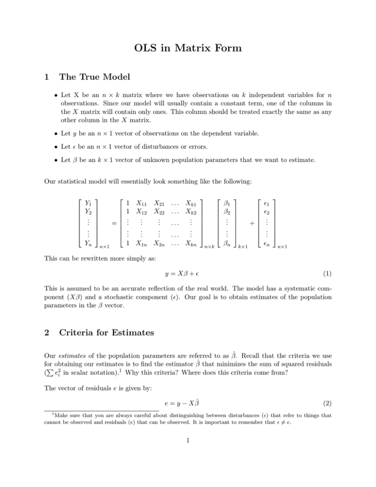
OLS in Matrix Form
1
The True Model
• Let X be an n × k matrix where we have observations on k independent variables for n
observations. Since our model will usually contain a constant term, one of the columns in
the X matrix will contain only ones. This column should be treated exactly the same as any
other column in the X matrix.
• Let y be an n × 1 vector of observations on the dependent variable.
• Let ² be an n × 1 vector of disturbances or errors.
• Let β be an k × 1 vector of unknown population parameters that we want to estimate.
Our statistical model will essentially look something like the following:








Y1
Y2
..
.
..
.
Yn












=



n×1
1 X11 X21
1 X12 X22
..
..
..
.
.
.
..
..
..
.
.
.
1 X1n X2n
. . . Xk1
. . . Xk2
..
...
.
..
...
.
. . . Xkn
















n×k
β1
β2
..
.
..
.
βn












+



k×1
²1
²2
..
.
..
.
²n








n×1
This can be rewritten more simply as:
y = Xβ + ²
(1)
This is assumed to be an accurate reflection of the real world. The model has a systematic component (Xβ) and a stochastic component (²). Our goal is to obtain estimates of the population
parameters in the β vector.
2
Criteria for Estimates
Our estimates of the population parameters are referred to as β̂. Recall that the criteria we use
for
P obtaining our estimates is to find the estimator β̂ that minimizes the sum of squared residuals
( e2i in scalar notation).1 Why this criteria? Where does this criteria come from?
The vector of residuals e is given by:
e = y − X β̂
1
(2)
Make sure that you are always careful about distinguishing between disturbances (²) that refer to things that
cannot be observed and residuals (e) that can be observed. It is important to remember that ² 6= e.
1
The sum of squared residuals (RSS) is e0 e.2


e1
 e2 


 .. 
¤
£
¤
£

e1 e2 . . . . . . en 1×n 
.
= e1 × e1 + e2 × e2 + . . . + en × en 1×1


 .. 
 . 
en n×1
(3)
It should be obvious that we can write the sum of squared residuals as:
e0 e = (y − X β̂)0 (y − X β̂)
= y 0 y − β̂ 0 X 0 y − y 0 X β̂ + β̂ 0 X 0 X β̂
= y 0 y − 2β̂ 0 X 0 y + β̂ 0 X 0 X β̂
(4)
where this development uses the fact that the transpose of a scalar is the scalar i.e. y 0 X β̂ =
(y 0 X β̂)0 = β̂ 0 X 0 y.
To find the β̂ that minimizes the sum of squared residuals, we need to take the derivative of Eq. 4
with respect to β̂. This gives us the following equation:
∂e0 e
∂ β̂
= −2X 0 y + 2X 0 X β̂ = 0
(5)
To check this is a minimum, we would take the derivative of this with respect to β̂ again – this
gives us 2X 0 X. It is easy to see that, so long as X has full rank, this is a positive definite matrix
(analogous to a positive real number) and hence a minimum.3
2
3
It is important to note that this is very different from ee0 – the variance-covariance matrix of residuals.
Here is a brief overview of matrix differentiaton.
∂a0 b
∂b0 a
=
=a
∂b
∂b
(6)
∂b0 Ab
= 2Ab = 2b0 A
∂b
(7)
when a and b are K×1 vectors.
when A is any symmetric matrix. Note that you can write the derivative as either 2Ab or 2b0 A.
∂2β 0 (X 0 y)
∂2β 0 X 0 y
=
= 2X 0 y
∂b
∂b
(8)
∂β 0 Aβ
∂β 0 X 0 Xβ
=
= 2Aβ = 2X 0 Xβ
∂b
∂b
(9)
and
when X 0 X is a K×K matrix. For more information, see Greene (2003, 837-841) and Gujarati (2003, 925).
2
From Eq. 5 we get what are called the ‘normal equations’.
(X 0 X)β̂ = X 0 y
(10)
Two things to note about the (X 0 X) matrix. First, it is always square since it is k × k. Second, it
is always symmetric.
Recall that (X 0 X) and X 0 y are known from our data but β̂ is unknown. If the inverse of (X 0 X) exists
(i.e. (X 0 X)−1 ), then pre-multiplying both sides by this inverse gives us the following equation:4
(X 0 X)−1 (X 0 X)β̂ = (X 0 X)−1 X 0 y
(11)
We know that by definition, (X 0 X)−1 (X 0 X) = I, where I in this case is a k × k identity matrix.
This gives us:
I β̂ = (X 0 X)−1 X 0 y
β̂ = (X 0 X)−1 X 0 y
(12)
Note that we have not had to make any assumptions to get this far! Since the OLS estimators in
the β̂ vector are a linear combination of existing random variables (X and y), they themselves are
random variables with certain straightforward properties.
3
Properties of the OLS Estimators
The primary property of OLS estimators is that they satisfy the criteria of minimizing the sum of
squared residuals. However, there are other properties. These properties do not depend on any
assumptions - they will always be true so long as we compute them in the manner just shown.
Recall the normal form equations from earlier in Eq. 10.
(X 0 X)β̂ = X 0 y
(13)
Now substitute in y = X β̂ + e to get
(X 0 X)β̂ = X 0 (X β̂ + e)
(X 0 X)β̂ = (X 0 X)β̂ + X 0 e
X 0e = 0
4
(14)
The inverse of (X 0 X) may not exist. If this is the case, then this matrix is called non-invertible or singular and is
said to be of less than full rank. There are two possible reasons why this matrix might be non-invertible. One, based
on a trivial theorem about rank, is that n < k i.e. we have more independent variables than observations. This is
unlikely to be a problem for us in practice. The other is that one or more of the independent variables are a linear
combination of the other variables i.e. perfect multicollinearity.
3
What does X 0 e

X11 X12
 X21 X22

 ..
..
 .
.

 ..
..
 .
.
Xk1 Xk2
look like?
. . . X1n
. . . X2n
..
..
.
.
..
..
.
.
. . . Xkn








e1
e2
..
.
..
.
en


 
 
 
=
 
 
 
X11 × e1 + X12 × e2 + . . . + X1n × en
X21 × e1 + X22 × e2 + . . . + X2n × en
..
.
..
.
Xk1 × e1 + Xk2 × e2 + . . . + Xkn × en


 
 
 
=
 
 
 
0
0
..
.
..
.
0








(15)
From X 0 e = 0, we can derive a number of properties.
1. The observed values of X are uncorrelated with the residuals.
X 0 e = 0 implies that for every column xk of X, x0k e = 0. In other words, each regressor
has zero sample correlation with the residuals. Note that this does not mean that X is uncorrelated with the disturbances; we’ll have to assume this.
If our regression includes a constant, then the following properties also hold.
2. The sum of the residuals is zero.
If there is a constant, then the first column in X (i.e. X1 ) will be a column of ones. This
0
means that for the first element in the
P X e vector (i.e. X11 × e1 + X12 × e2 + . . . + X1n × en )
to be zero, it must be the case that
ei = 0.
3. The sample mean of the residuals is zero.
P
This follows straightforwardly from the previous property i.e. e =
ei
n
= 0.
4. The regression hyperplane passes through the means of the observed values (X
and y).
This follows from the fact that e = 0. Recall that e = y − X β̂. Dividing by the number
of observations, we get e = y − xβ̂ = 0. This implies that y = xβ̂. This shows that the
regression hyperplane goes through the point of means of the data.
5. The predicted values of y are uncorrelated with the residuals.
The predicted values of y are equal to X β̂ i.e. ŷ = X β̂. From this we have
ŷ 0 e = (X β̂)0 e = b0 X 0 e = 0
(16)
This last development takes account of the fact that X 0 e = 0.
6. The mean of the predicted Y’s for the sample will equal the mean of the observed
Y’s i.e. ŷ = y.
4
These properties always hold true. You should be careful not to infer anything from the residuals
about the disturbances. For example, you cannot infer that the sum of the disturbances is zero or
that the mean of the disturbances is zero just because this is true of the residuals - this is true of
the residuals just because we decided to minimize the sum of squared residuals.
Note that we know nothing about β̂ except that it satisfies all of the properties discussed above.
We need to make some assumptions about the true model in order to make any inferences regarding
β (the true population parameters) from β̂ (our estimator of the true parameters). Recall that β̂
comes from our sample, but we want to learn about the true parameters.
4
The Gauss-Markov Assumptions
1. y = Xβ + ²
This assumption states that there is a linear relationship between y and X.
2. X is an n × k matrix of full rank.
This assumption states that there is no perfect multicollinearity. In other words, the columns
of X are linearly independent. This assumption is known as the identification condition.
3. E[²|X] = 0



E

²1 |X
²2 |X
..
.


 
 
=
 
²n |X
E(²1 )
E(²2 )
..
.
E(²n )


 
 
=
 
0
0
..
.





(17)
0
This assumption - the zero conditional mean assumption - states that the disturbances average
out to 0 for any value of X. Put differently, no observations of the independent variables
convey any information about the expected value of the disturbance. The assumption implies
that E(y) = Xβ. This is important since it essentially says that we get the mean function
right.
4. E(²²0 |X) = σ 2 I
This captures the familiar assumption of homoskedasticity and no autocorrelation. To see
why, start with the following:


²1 |X
 ²2 |X  £
¤


E(²²0 |X) = E  .  ²1 |X ²2 |X . . . ²n |X]
(18)
 .. 
²n |X
5
which is the same as:



E(²²0 |X) = E 

²21 |X
²2 ²1 |X
..
.
²1 ²2 |X
²22 |X
..
.
. . . ²1 ²n |X
. . . ²2 ²n |X
..
..
.
.
²n ²1 |X ²n ²2 |X . . . ²2n |X





(19)
which is the same as:



E(²²0 |X) = 

E[²21 |X] E[²1 ²2 |X] . . . E[²1 ²n |X]
E[²2 ²1 |X] E[²22 |X] . . . E[²2 ²n |X]
..
..
..
..
.
.
.
.
E[²n ²1 |X] E[²n ²2 |X] . . . E[²2n |X]





(20)
The assumption of homoskedasticity states that the variance of ²i is the same (σ 2 ) for all i
i.e. var[²i |X] = σ 2 ∀ i. The assumption of no autocorrelation (uncorrelated errors) means
that cov(²i , ²j |X) = 0 ∀ i 6= j i.e. knowing something about the disturbance term for one
observation tells us nothing about the disturbance term for any other observation. With these
assumptions, we have:
 2

σ
0 ... 0
 0 σ2 . . . 0 


E(²²0 |X) =  .
(21)
..
..
.. 
 ..
.
.
. 
0
0
. . . σ2
Finally, this can be rewritten as:



E(²²0 |X) = σ 2 


1 0 ... 0
0 1 ... 0 

2
.. .. .. ..  = σ I
. . . . 
0 0 ... 1
(22)
Disturbances that meet the two assumptions of homoskedasticity and no autocorrelation are
referred to as spherical disturbances. We can compactly write the Gauss-Markov assumptions
about the disturbances as:
Ω = σ2I
(23)
where Ω is the variance-covariance matrix of the disturbances i.e. Ω = E[²²0 ].
5. X may be fixed or random, but must be generated by a mechanism that is unrelated to ².
6. ²|X ∼ N [0, σ 2 I]
This assumption is not actually required for the Gauss-Markov Theorem. However, we often
assume it to make hypothesis testing easier. The Central Limit Theorem is typically evoked
to justify this assumption.
6
5
The Gauss-Markov Theorem
The Gauss-Markov Theorem states that, conditional on assumptions 1-5, there will be no other
linear and unbiased estimator of the β coefficients that has a smaller sampling variance. In other
words, the OLS estimator is the Best Linear, Unbiased and Efficient estimator (BLUE). How do
we know this?
Proof that β̂ is an unbiased estimator of β.
We know from earlier that β̂ = (X 0 X)−1 X 0 y and that y = Xβ + ². This means that
β̂ = (X 0 X)−1 X 0 (Xβ + ²)
β̂ = β + (X 0 X)−1 X 0 ²
(24)
since (X 0 X)−1 X 0 X = I. This shows immediately that OLS is unbiased so long as either (i) X is
fixed (non-stochastic) so that we have:
E[β̂] = E[β] + E[(X 0 X)−1 X 0 ²]
= β + (X 0 X)−1 X 0 E[²]
(25)
where E[²] = 0 by assumption or (ii) X is stochastic but independent of ² so that we have:
E[β̂] = E[β] + E[(X 0 X)−1 X 0 ²]
= β + (X 0 X)−1 E[X 0 ²]
(26)
where E(X 0 ²) = 0.
Proof that β̂ is a linear estimator of β.
From Eq. 24, we have:
β̂ = β + (X 0 X)−1 X 0 ²
(27)
Since we can write β̂ = β + A² where A = (X 0 X)−1 X 0 , we can see that β̂ is a linear function of the
disturbances. By the definition that we use, this makes it a linear estimator (See Greene (2003, 45).
Proof that β̂ has minimal variance among all linear and unbiased estimators
See Greene (2003, 46-47).
7
6
The Variance-Covariance Matrix of the OLS Estimates
We can derive the variance-covariance matrix of the OLS estimator, β̂.
E[(β̂ − β)(β̂ − β)0 ] = E[((X 0 X)−1 X 0 ²)((X 0 X)−1 X 0 ²)0 ]
= E[(X 0 X)−1 X 0 ²²0 X(X 0 X)−1 ]
(28)
where we take advantage of the fact that (AB)0 = B 0 A0 i.e. we can rewrite (X 0 X)−1 X 0 ² as
²0 X(X 0 X)−1 . If we assume that X is non-stochastic, we get:
E[(β̂ − β)(β̂ − β)0 ] = (X 0 X)−1 X 0 E[²²0 ]X(X 0 X)−1
(29)
From Eq. 22, we have E[²²0 ] = σ 2 I. Thus, we have:
E[(β̂ − β)(β̂ − β)0 ] = (X 0 X)−1 X 0 (σ 2 I)X(X 0 X)−1
= σ 2 I(X 0 X)−1 X 0 X(X 0 X)−1
= σ 2 (X 0 X)−1
(30)
We estimate σ 2 with σ̂ 2 , where:
σ̂ 2 =
e0 e
n−k
(31)
To see the derivation of this, see Greene (2003, 49).
What does the variance-covariance matrix of the OLS estimator look like?

var(β̂1 )
cov(β̂1 , β̂2 ) . . . cov(β̂1 , β̂k )
 cov(β̂2 , β̂1 )
var(β̂2 )
. . . cov(β̂2 , β̂k )

E[(β̂ − β)(β̂ − β)0 ] = 
.
.
..
..
..
..

.
.
cov(β̂k , β̂1 ) cov(β̂k , β̂2 ) . . .
var(β̂k )





(32)
As you can see, the standard errors of the β̂ are given by the square root of the elements along the
main diagonal of this matrix.
6.1
Hypothesis Testing
Recall Assumption 6 from earlier, which stated that ²|X ∼ N [0, σ 2 I]. I had stated that this
assumption was not necessary for the Gauss-Markov Theorem but was crucial for testing inferences
about β̂. Why? Without this assumption, we know nothing about the distribution of β̂. How does
this assumption about the distribution of the disturbances tell us anything about the distribution of
β̂? Well, we just saw in Eq. 27 that the OLS estimator is just a linear function of the disturbances.
By assuming that the disturbances have a multivariate normal distribution i.e.
² ∼ N [0, σ 2 I]
8
(33)
we are also saying that the OLS estimator is also distributed multivariate normal i.e.
β̂ ∼ N [β, σ 2 (X 0 X)−1 ]
(34)
but where the mean is β and the variance is σ 2 (X 0 X)−1 . It is this that allows us to conduct the
normal hypothesis tests that we are familiar with.
7
Robust (Huber of White) Standard Errors
Recall from Eq. 29 that we have:
var − cov(β̂) = (X 0 X)−1 X 0 E[²²0 ]X(X 0 X)−1
= (X 0 X)−1 (X 0 ΩX)(X 0 X)−1
(35)
This helps us to make sense of White’s heteroskedasticity consistent standard errors.5
Recall that heteroskedasticity does not cause problems for estimating the coefficients; it only causes
problems for getting the ‘correct’ standard errors. We can compute β̂ without making any assumptions about the disturbances i.e. β̂OLS = (X 0 X)−1 X 0 y. However, to get the results of the
Gauss Markov Theorem (things like E[β̂] = β etc.) and to be able to conduct hypothesis tests
(β̂ ∼ N [β, σ 2 (X 0 X)−1 ]), we need to make assumptions about the disturbances. One of the assumptions is that E[ee0 ] = σ 2 I. This assumption includes the assumption of homoskedasticity –
var[²i |X] = σ 2 ∀ i. However, it is not always the case that the variance will be the same for all
observations i.e. we have σi2 instead of σ 2 . Basically, there may be many reasons why we are
better at predicting some observations than others. Recall the variance-covariance matrix of the
disturbance terms from earlier:


E[²21 |X] E[²1 ²2 |X] . . . E[²1 ²n |X]
 E[²2 ²1 |X] E[²2 |X] . . . E[²2 ²n |X] 
2


E(²²0 |X) = Ω = 
(36)

..
..
..
..


.
.
.
.
E[²n ²1 |X] E[²n ²2 |X] . . .
E[²2n |X]
If we retain the assumption of no autocorrelation, this can be rewritten as:

 2
σ1 0 . . . 0
 0 σ2 . . . 0 
2


E(²²0 |X) = Ω =  .
..
..
.. 
 ..
.
.
. 
0 0 . . . σn2
(37)
Basically, the main diagonal contains n variances of ²i . The assumption of homoskedasticity states
that each of these n variances are the same i.e. σi2 = σ 2 . But this is not always an appropriate
5
As we’ll see later in the semester, it also helps us make sense of Beck and Katz’s panel-corrected standard errors.
9
assumption to make. Our OLS standard errors will be incorrect insofar as:
X 0 E[²²0 ]X 6= σ 2 (X 0 X)
(38)
Note that our OLS standard errors may be too big or too small. So, what can we do if we suspect
that there is heteroskedasticity?
Essentially, there are two options.
1. Weighted Least Squares: To solve the problem, we just need to find something that is
proportional to the variance. We might not know the variance for each observation, but
if we know something about where it comes from, then we might know something that is
proportional to it. In effect, we try to model the variance. Note that this only solves the
problem of heteroskedasticity if we assume that we have modelled the variance correctly - we
never know if this is true or not.
2. Robust standard errors (White 1980): This method treats heteroskedasticity as a nuisance
rather than something to be modelled.
How do robust standard errors work? We never observe disturbances (²) but we do observe residuals
(e). While each individual residual (ei ) is not going to be a very good estimator of the corresponding
disturbance (²i ), White (1980) showed that X 0 ee0 X is a consistent (but not unbiased) estimator of
X 0 E[²²0 ]X.6
Thus, the variance-covariance matrix of the coefficient vector from the White estimator is:
var − cov(β̂) = (X 0 X)−1 X 0 ee0 X(X 0 X)−1
(39)
rather than:
var − cov(β̂) = X 0 X)−1 X 0 ²²0 X(X 0 X)−1
= (X 0 X)−1 X 0 (σ 2 I)X(X 0 X)−1
(40)
from the normal OLS estimator.
White (1980) suggested that we could test for the presence of heteroskedasticity by examining the
extent to which the OLS estimator diverges from his own estimator. White’s test is to regress
the squared residuals (e2i ) on the terms in X 0 X i.e. on the squares and the cross-products of the
independent variables. If the R2 exceeds a critical value (nR2 ∼ χ2k ), then heteroskedasticity causes
problems. At that point use the White estimator (assuming your sample is sufficiently large). Neal
Beck suggests that, by and large, using the White estimator can do little harm and some good.
6
It is worth remembering that X 0 ee0 X is a consistent (but not unbiased) estimator of X 0 E[²²0 ]X since this means
that robust standard errors are only appropriate when the sample is relatively large (say, greater than 100 degrees of
freedom).
10
8
Partitioned Regression and the Frisch-Waugh-Lovell Theorem
Imagine that our true model is:
y = X1 β1 + X2 β2 + ²
(41)
In other words, there are two sets of independent variables. For example, X1 might contain some
independent variables (perhaps also the constant) whereas X2 contains some other independent
variables. The point is that X1 and X2 need not be two variables only. We will estimate:
y = X1 β̂1 + X2 β̂2 + e
(42)
Say, we wanted to isolate the coefficients associated with X2 i.e. β̂2 . The normal form equations
will be:7
¸ · 0 ¸
· 0
¸·
X1 y
βˆ1
(1)
X1 X1 X10 X2
=
(43)
X20 y
(2)
X20 X1 X20 X2
βˆ2
First, let’s solve for βˆ1 .
(X10 X1 )βˆ1 + (X10 X2 )βˆ2 = X10 y
(X10 X1 )βˆ1 = X10 y − (X10 X2 )βˆ2
βˆ1 = (X 0 X1 )−1 X 0 y − (X 0 X1 )−1 X 0 X2 βˆ2
1
1
1
1
βˆ1 = (X10 X1 )−1 X10 (y − X2 βˆ2 )
8.1
(44)
Omitted Variable Bias
The solution shown in Eq. 44 is the set of OLS coefficients in the regression of y on X1 , i.e,
(X10 X1 )−1 X10 y, minus a correction vector (X10 X1 )−1 X10 X2 βˆ2 . This correction vector is the equation
for omitted variable bias. The first part of the correction vector up to βˆ2 , i.e. (X10 X1 )−1 X10 X2 , is
just the regression of the variables in X2 done separately and then put together into a matrix on all
the variables in X1 . This will only be zero if the variables in X1 are linearly unrelated (uncorrelated
or orthogonal) to the variables in X2 . The correction vector will also be zero if βˆ2 = 0 i.e. if X2
variables have no impact on y. Thus, you can ignore all potential omitted variables that are either
(i) unrelated to the included variables or (ii) unrelated to the dependent variable. Any omitted
variables that do not meet these conditions will change your estimates of βˆ1 if they were to be
included.
Greene (2003, 148) writes the omitted variable formula slightly differently. He has
E[b1 ] = β1 + P1.2 β2
(45)
where P1.2 = (X10 X1 )−1 X10 X2 , where b1 is the coefficient vector of a regression omitting the X2
7
To see this, compare with Eq. 10.
11
matrix, and β1 and β2 are the true coefficient vectors from a full regression including both X1 and
X2 .
8.2
The Residual Maker and the Hat Matrix
Before going any further, I introduce some useful matrices. Note that:
e = y − X β̂
= y − X(X 0 X)−1 X 0 y
= (I − X(X 0 X)−1 X 0 )y
= My
(46)
where M is called the residual maker since it makes residuals out of y. M is a square matrix and
is idempotent. A matrix A is idempotent if A2 = AA = A.
MM
= (I − X(X 0 X)−1 X 0 )(I − X(X 0 X)−1 X 0 )
= I 2 − 2X(X 0 X)−1 X 0 + X(X 0 X)−1 X 0 X(X 0 X)−1 X 0
= I − 2X(X 0 X)−1 X 0 + X(X 0 X)−1 X 0
= I − X(X 0 X)−1 X 0
= M
(47)
This will prove useful. The M matrix also has the properties that M X = 0 and M e = e.
A related matrix is the hat matrix (H) which makes ŷ our of y. Note that:
ŷ = y − e = [I − M ]y = Hy
(48)
H = X(X 0 X)−1 X 0
(49)
where:
Greene refers to this matrix as P, but he is the only one that does this.
8.3
Frisch-Waugh-Lovell Theorem
So far we have solved for βˆ1 .
βˆ1 = (X10 X1 )−1 X10 (y − X2 βˆ2 )
12
(50)
Now we insert this into (2) of Eq. 43. This gives us
X20 y = X20 X1 (X10 X1 )−1 X10 y − X20 X1 (X10 X1 )−1 X10 X2 βˆ2 + X20 X2 βˆ2
X20 y − X20 X1 (X10 X1 )−1 X10 y = X20 X2 βˆ2 − X20 X1 (X10 X1 )−1 X10 X2 βˆ2
X 0 y − X 0 X1 (X 0 X1 )−1 X 0 y = [X 0 X2 − X 0 X1 (X 0 X1 )−1 X 0 X2 ]βˆ2
2
2
1
1
0
0
0
−1 0
X2 y − X2 X1 (X1 X1 ) X1 y
X20 y − X20 X1 (X10 X1 )−1 X10 y
(X20 − X20 X1 (X10 X1 )−1 X10 )y
X20 (I − X1 (X10 X1 )−1 X10 )y
2
=
=
=
=
βˆ2 =
=
2
1
1
0
0
0
−1 0
[(X2 − X2 X1 (X1 X1 ) X1 )X2 ]βˆ2
[X20 (I − X1 (X10 X1 )−1 X10 )X2 ]βˆ2
[X20 (I − X1 (X10 X1 )−1 X10 )X2 ]βˆ2
[X20 (I − X1 (X10 X1 )−1 X10 )X2 ]βˆ2
[X20 (I − X1 (X10 X1 )−1 X10 )X2 ]−1 X20 (I
(X20 M1 X2 )−1 (X20 M1 y)
− X1 (X10 X1 )−1 X10 )y
(51)
Recall that M is the residual maker. In this case, M1 makes residuals for regressions on the X1
variables: M1 y is the vector of residuals from regressing y on the X1 variables and M1 X2 is the
matrix made up of the column by column residuals of regressing each variable (column) in X2 on
all the variables in X1 .
Because M is both idempotent and symmetric, we can rewrite Eq. 51 as
0
0
βˆ2 = (X2∗ X2 )−1 X2∗ y ∗
(52)
where X2∗ = M1 X2 and y ∗ = M1 y.
From this it is easy to see that βˆ2 can be obtained from regressing y ∗ on X2∗ (you’ll get good at
spotting regressions i.e. equations of the (X 0 X)−1 X 0 y form. The starred variables are just the
residuals of the variables (y or X2 ) after regressing them on the X1 variables.
This leads to the Frisch-Waugh-Lovell Theorem: In the OLS regression of vector y on two sets
of variables, X1 and X2 , the subvector βˆ2 is the set of coefficients obtained when the residuals from
a regression of y on X1 alone are regressed on the set of residuals obtained when each column of
X2 is regressed on X1 .
We’ll come back to the FWL Theorem when we look at fixed effects models.
8.4
Example
Imagine we have the following model.
Y = β0 + β1 X1 + β2 X2 + β3 X3 + ²
(53)
If we regressed Y on X1 , X2 , and X3 , we would get βˆ1 , βˆ2 , βˆ3 . We could get these estimators
differently. Say we partitioned the variables into (i) X1 and (ii) X2 and X3 .
Step 1: regress Y on X1 and obtain residuals (e1) i.e. M1 y.
13
Step
Step
Step
Step
2:
3:
4:
5:
regress X2 on X1 and obtain residuals (e2) i.e. first column of M1 X2 .
regress X3 on X1 and obtain residuals (e3) i.e. second column of M1 X2 .
regress e1 on e2 and e3 i.e. regress M1 y on M1 X2 .
the coefficient on e2 will be βˆ2 and the coefficient on e3 will be βˆ3 .
Steps 2 and 3 are called partialing out or netting out the effect of X1 . For this reason, the coefficients
in multiple regression are often called partial regression coefficients. This is what it means to say
we are holding the X1 variables constant in the regression.
So the difference between regressing Y on both X1 and X2 instead of on just X2 is that in the
first case we first regress both the dependent variables and all the X2 variables separately on X1
and then regress the residuals on each other, but in the second case we just regress y on the X2
variables.
14